2.4. Plotting 1D arrays
The plotting of 1D arrays option and plot handling is the main feature and purpose of the IMASViz.
This section describes the basics of plotting a 1D array, stored in the IDS, and how to handle the existing plots.
2.4.1. Plotting a single 1D array to plot figure
The procedure to plot 1D array is as follows:
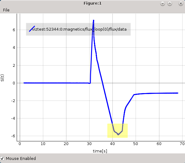
Navigate through the magnetics IDS and search for the node containing FLT_1D data, for example magnetics.flux_loop[0].flux.data. Plottable FLT_1D nodes are colored blue (array length > 0).
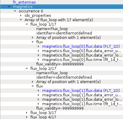
Example of plottable FLT_1D node.
By clicking on the node the preview plot will be displayed in the Preview Plot, located in the main window. This feature helps to quickly check how the data, stored in the FLT_1D, looks when plotted.

Preview Plot
Right-click on the magnetics.flux_loop[0].flux.data (FLT_1D) node.
From the pop-up menu, select the command Plot ids.magnetics.flux_loop[0].flux.data to
 ->
figure
->
figure  -> New
  .
.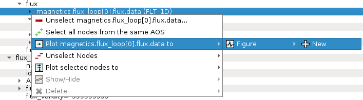
Navigating through right-click menu to plot data to plot figure.
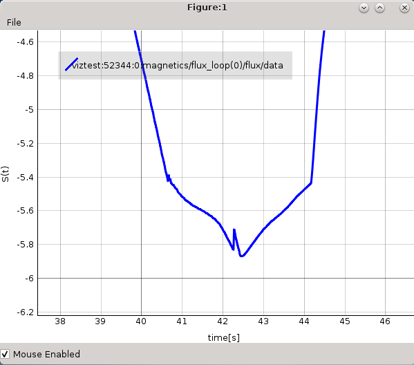
The plot should display in plot figure as shown in the image below.
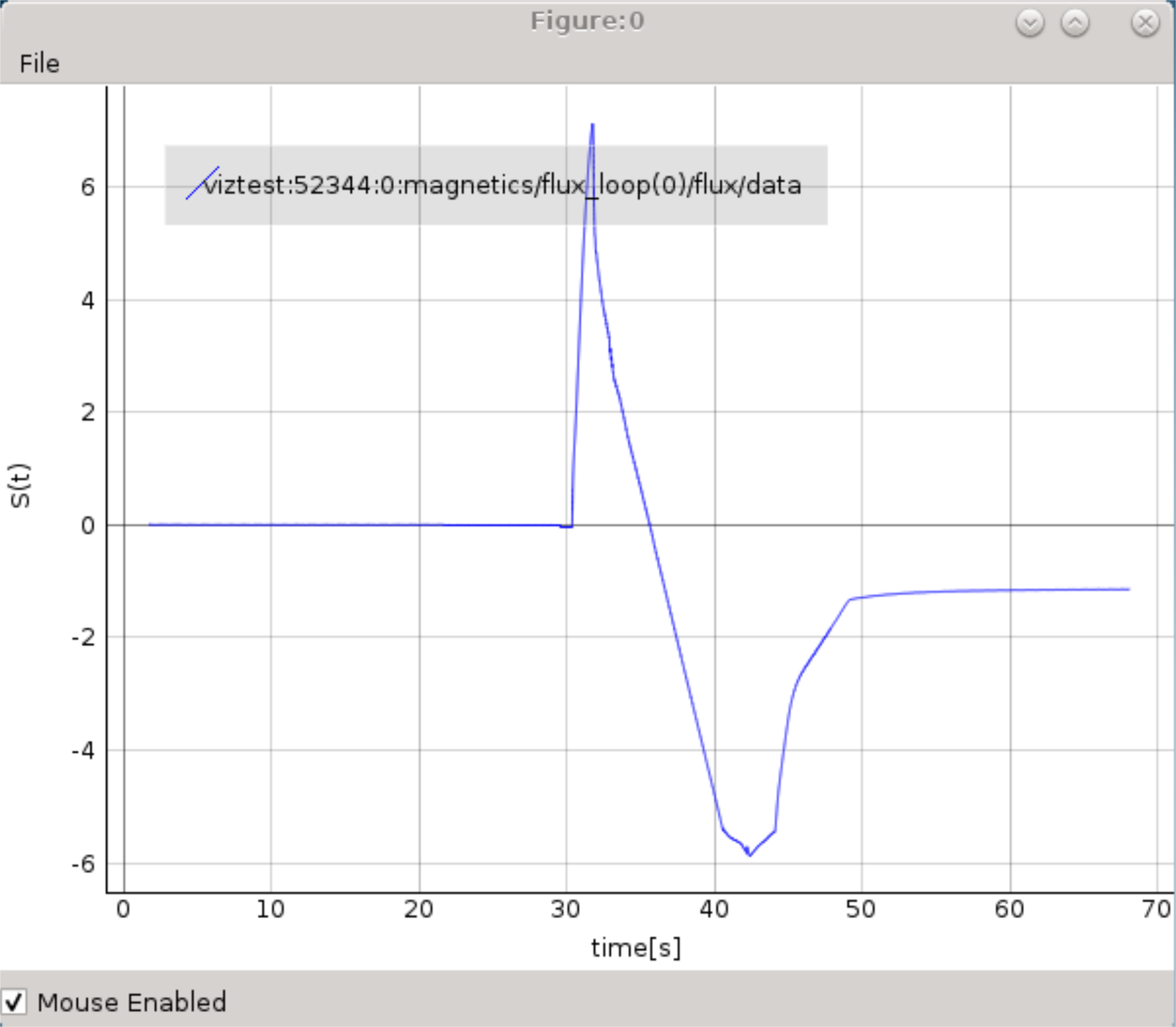
Basic plot figure display.
2.4.1.1. Basic plot display features
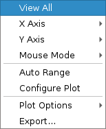
The below features are available for any plot display. Most of them are available in the right-click menu.
Note
Term Plot Display is used for any base subwindow for displaying plots. Following that the Plot Figure contains a single Plot Display, while Table Plot View and Stacked Plot View consist of multiple Plot Displays.
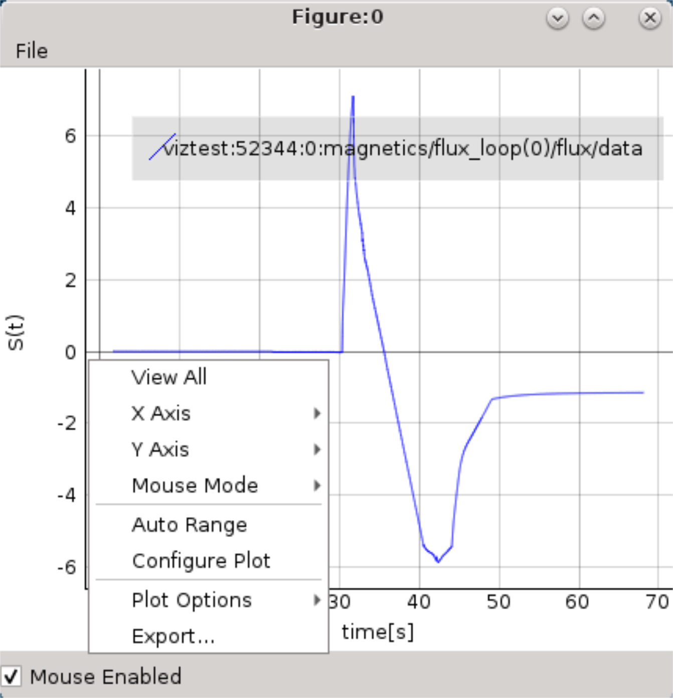
Plot display window right-click menu.
2.4.1.1.2. Auto Range
Similar to View All feature with the difference that it shows
plot area between values X_min -> X_max and Y_min -> Y_max,
without additional “plot margins” on the sides.
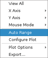
Auto Range feature in the right-click menu.
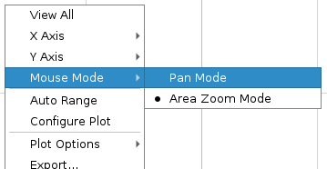
2.4.1.1.3. Left Mouse Button Mode Change
Change between Pan Mode (move plot around) and Area Zoom Mode (choose selectable area to zoom into).
2.4.1.1.4. Axis options
X and Y axis range, inverse, mouse enable/disable options and more.
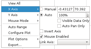
Axis Options feature in the right-click menu.
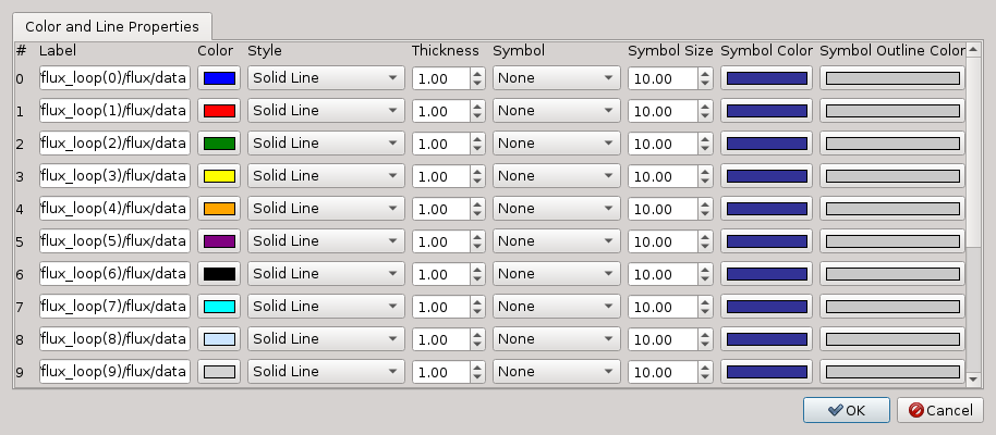
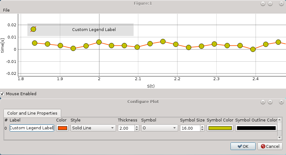
2.4.1.1.5. Plot Configuration and Customization
Setting color and line properties of plots shown in the Plot Display.
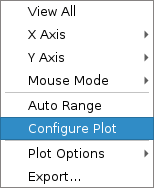
Configure Plot feature in the right-click menu.
Each plot can be customized. By selecting this feature a separate GUI window will open, listing all plots within the plot display window and their properties that can be customized.
2.4.1.1.6. Plot options
Enable/Disable grid, log scale and more.
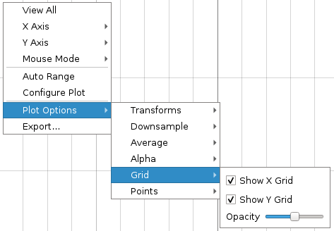
Plot Options feature in the right-click menu.
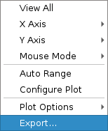
2.4.1.1.7. Export feature
- The Plot Display scene can be exported to:
image file (PNG, JPG, …). A total of 16 image formats are supported.
scalable vector graphics (SVG) file
matplotlib window
CSV file
HDF5 file
Export feature in the right-click menu.
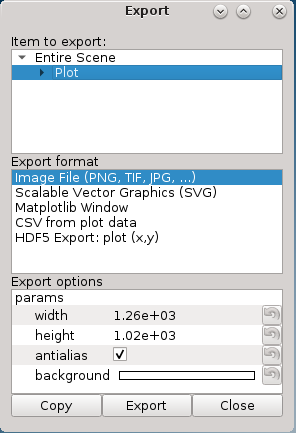
Export GUI window.
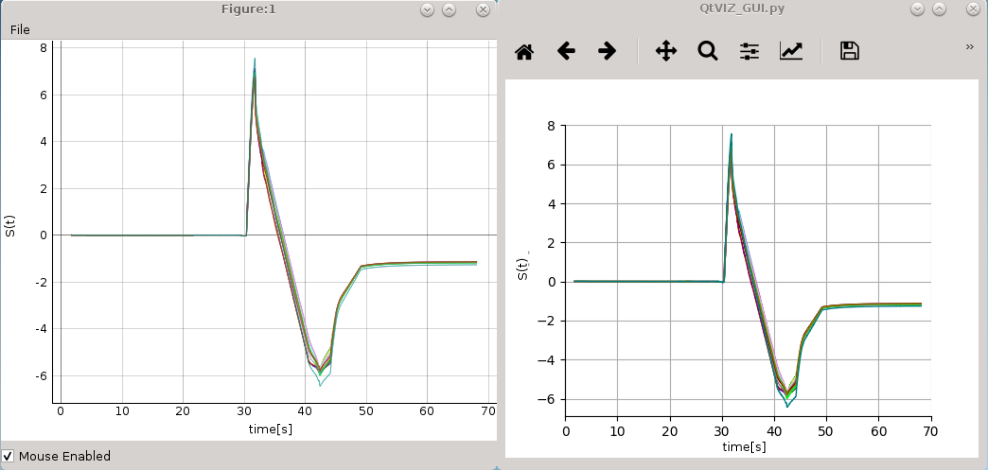
Comparison of IMASViz Plot Figure and matplotlib window
2.4.2. Adding a plot to existing figure
The procedure of adding a plot to an already existing figure is as follows:
From the previous navigation tree, navigate to the wanted node, for example ids.magnetics.flux_loop[16].flux.data
Right-click on the node.
From the pop-up menu, navigate and select Plot <node name> to
->
Figure -> Figure:0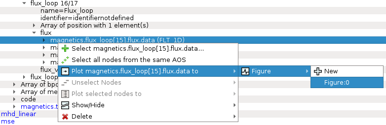
Plotting to existing figure.
The plot will be added to the selected existing plot as shown in the image below.
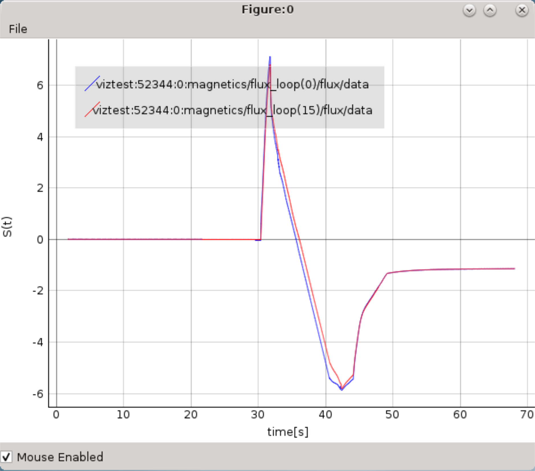
Plotting to existing figure - result.
2.4.3. Comparing plots between two IDS databases
IMASViz allows comparing of FLT_1D arrays between two different IDS databases (different shots too). The procedure is very similar to the one presented in the section Adding a plot to existing figure:
Open another IMAS database, same as shown in section Loading IDS from IMAS local data source. In this manual this will be demonstrated using IDS with shot 52682 and run 0 parameters.
Manual IDS case
parameters
values
User name
g2penkod
IMAS database name
viztest
Shot number
52682
Run number
0
Load occurrence 0 of magnetics IDS
Navigate through the IDS search for the wanted node, for example ids.magnetics.flux_loop[0].flux.data.
Right-click on the node.
From the pop-up menu, navigate and select Plot <node name> to
->
Figure -> Figure:0
The plot will be added to the existing plot as shown in the image below.
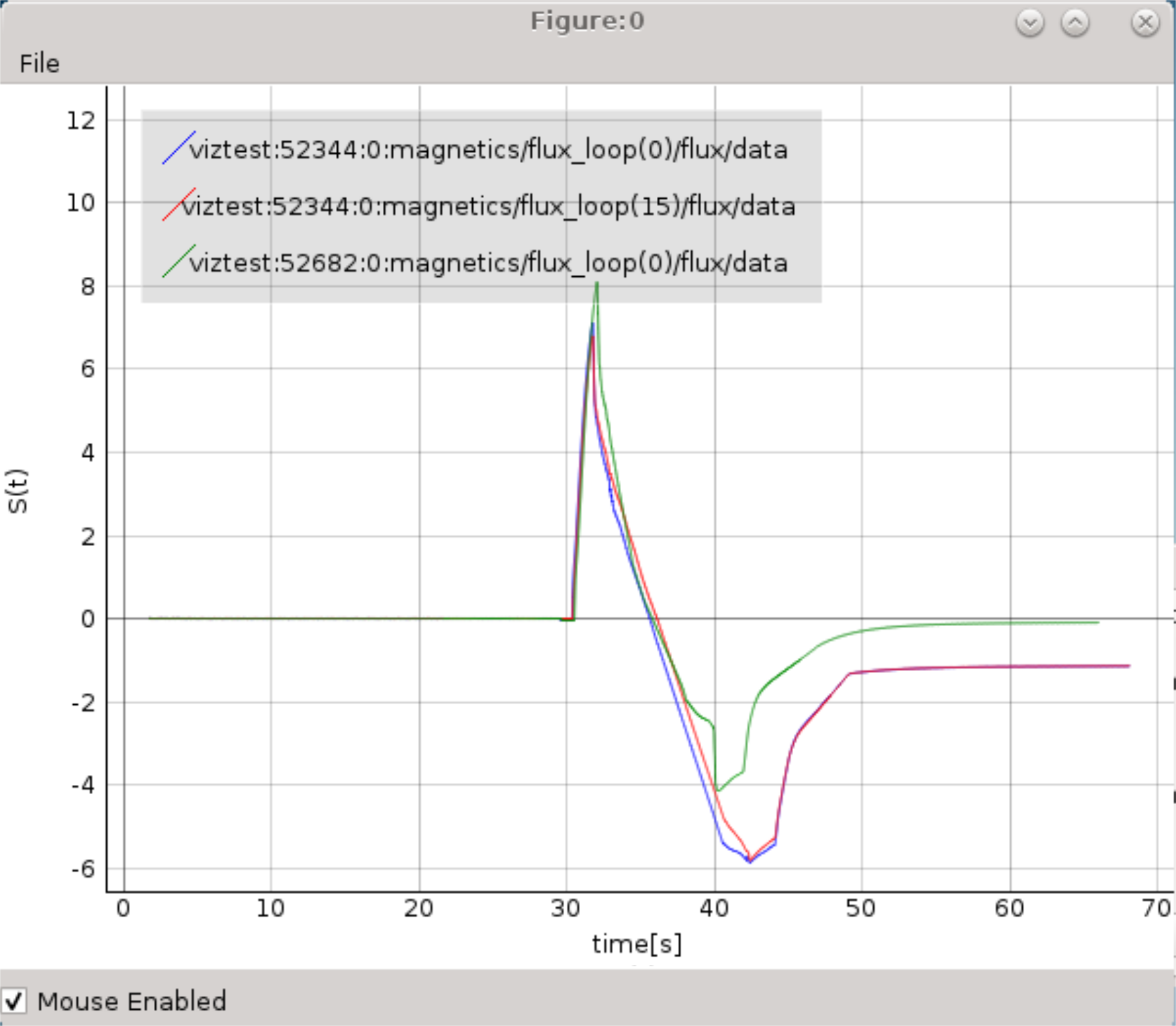
Plotting from other IDS to existing figure - result.
2.4.4. Plotting a selection of 1D arrays to figure
The procedure of 1D arrays selection and plotting to figure is as follows:
In main tree view window set a selection of nodes holding 1D arrays.
Note
How to create a selection of arrays is described in section Node selection features.
When finished with node selection, either: - right-click on any FLT_1D node, or - click Node Selection menu on menubar of the main tree view window.
From the pop-up menu, navigate and select Plot selected nodes to
 ->
Figure -> New ->
This IMAS database
->
Figure -> New ->
This IMAS database  .
.Note
The same procedure applies plotting the selection to an existing figure.
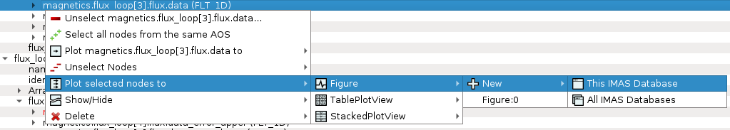
Plotting selection to a new figure using selection from the currently opened IDS database.
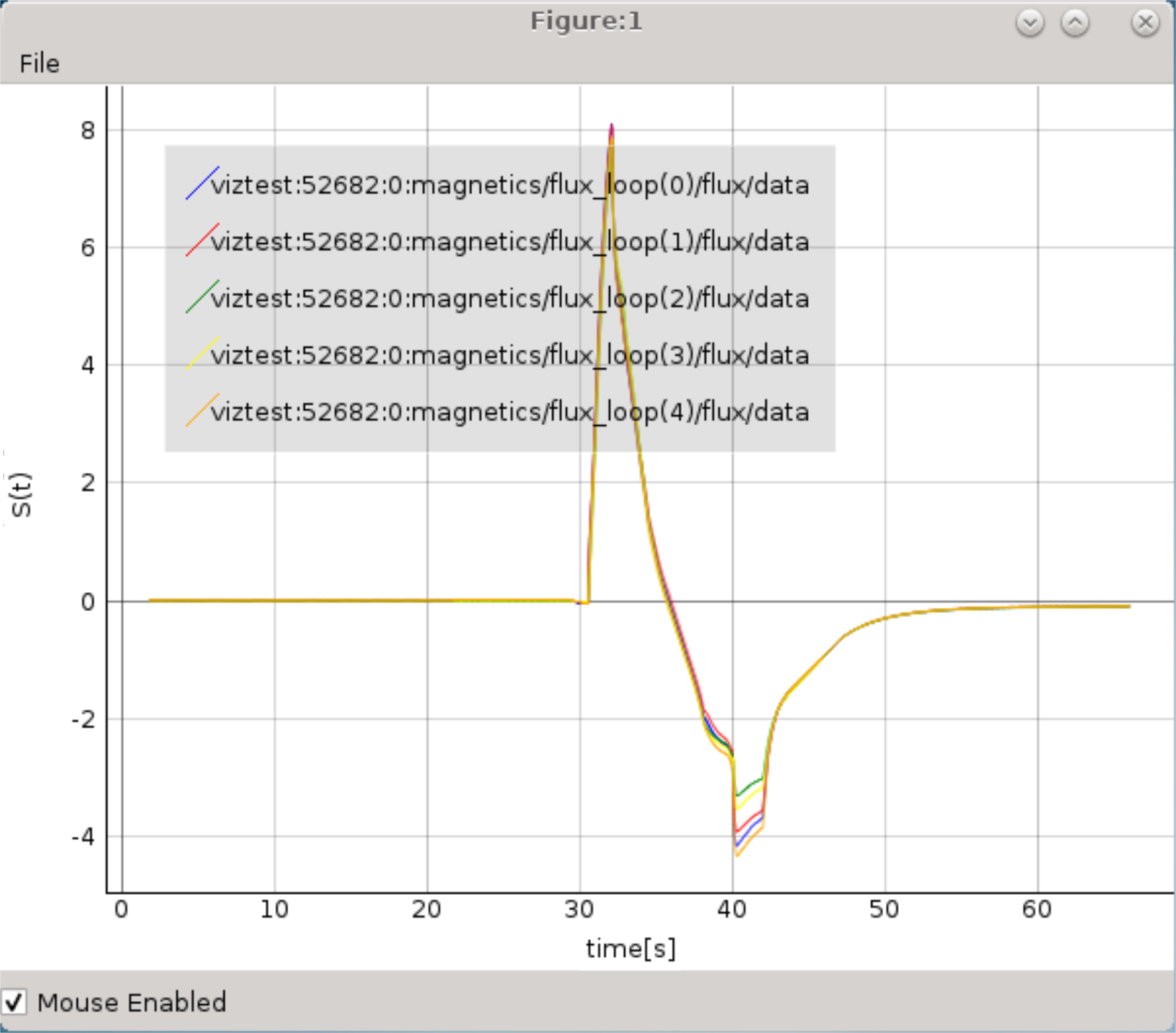
Example of plot figure, created by plotting data from node selection.
2.4.5. Plotting 1D array as a function of coordinate1 along the time axis
One of the IMASViz features is plotting coordinate along the time axis. This is allowed for IDS nodes, located within time_slice[:] structure, and it is already set as a default plotting feature for such arrays.
The procedure to plot such 1D array is quite identical as in section Plotting a single 1D array to plot figure. The procedure is described and demonstrated on equilibrium.time_slice[0].profiles_1d.phi (Torodial Flux) array.
Navigate through the equilibrium IDS and search for the time slice node containing FLT_1D data, for example equilibrium.time_slice[0].profiles_1d.phi.
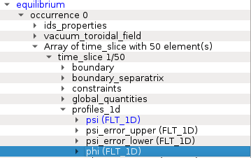
Example of plottable FLT_1D time slice node.
Right-click on the equilibrium.time_slice[0].profiles_1d.phi (FLT_1D) node.
From the pop-up menu, select the command Plot equilibrium.time_slice[0].profiles_1d.phi to
-> figure ->
New .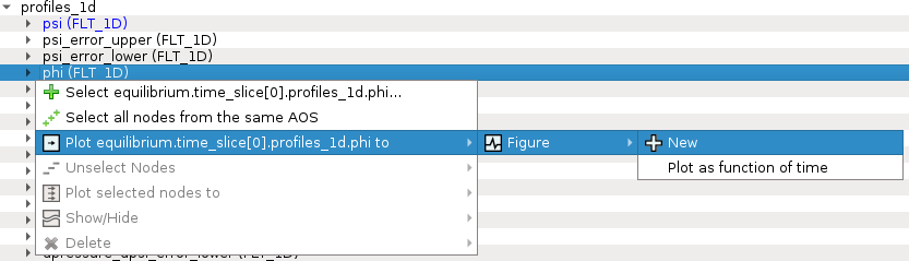
Navigating through right-click menu to plot data to plot figure.
The plot should display in plot figure as shown in the image below. Note that coordinate1 = ids.equilibrium.time_slice[0].profiles_1d.psi for this FLT_1D data array.
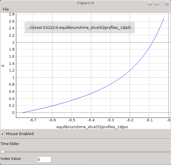
Time slice plot figure display. The data are represented as a function of coordinate1 (ids.equilibrium.time_slice[0].profiles_1d.psi) for the first phi time slice (ids.equilibrium.time_slice[0].profiles_1d.phi).
The time slider allows you to move along the time axis and the plot will change accordingly.
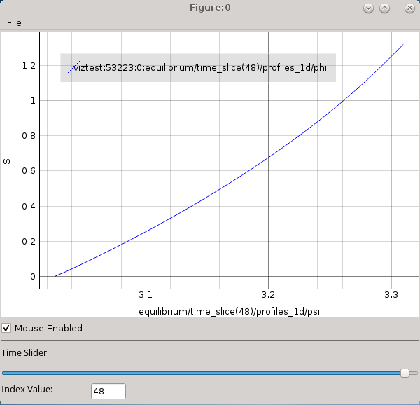
Time slice plot figure display for ids.equilibrium.time_slice[48].profiles_1d.phi. The data are represented as a function of coordinate1 (ids.equilibrium.time_slice[48].profiles_1d.psi).
Note
Adding a plot (presented in Adding a plot to existing figure) to such existing plot might not work as expected, as the sliding through indexes works directly only the last added plot.
2.4.6. Plotting 1D arrays at index as a function of the time
One of the IMASViz features is plotting array values at certain index as a function of time. This is allowed for IDS nodes, located within time_slice[:] structure, and it is already set as a default plotting feature for such arrays.
The procedure is described and demonstrated on equilibrium.time_slice[0].profiles_1d.f (Torodial Flux) array.
Navigate through the equilibrium IDS and search for the time slice node containing FLT_1D data, for example equilibrium.time_slice[0].profiles_1d.f.
Example of plottable FLT_1D time slice node.
Right-click on the equilibrium.time_slice[0].profiles_1d.f (FLT_1D) node.
From the pop-up menu, select the command Plot equilibrium.time_slice[0].profiles_1d.f to
-> figure ->
New .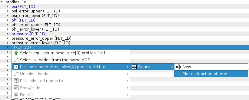
Navigating through right-click menu to plot data to plot figure.
The plot should display in plot figure as shown in the image below. Note that Y-axis values are an array of equilibrium.time_slice[:].profiles_1d.f[0] values through all time slices (marked by [:]) and X-axis values are time values found in equilibrium.time.
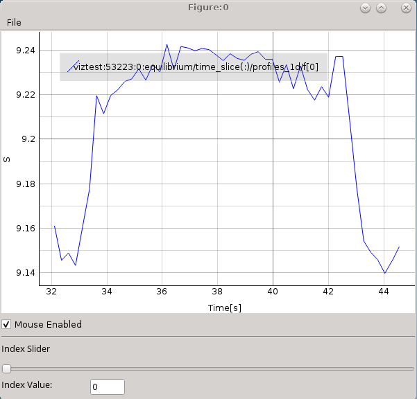
Plot as a function of time. Y-axis values are an array of equilibrium.time_slice[:].profiles_1d.f[0] values through all time slices (marked by [:]) and X-axis values are time values found in equilibrium.time.
The time slider allows you to move along the array index and the plot will change accordingly.
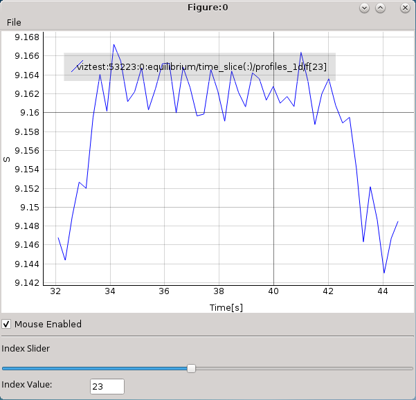
Plot as a function of time. Y-axis values are an array of equilibrium.time_slice[:].profiles_1d.f[23] values through all time slices (marked by [:]) and X-axis values are time values found in equilibrium.time node (array of FLT_1D values).
Note
Adding a plot (presented in Adding a plot to existing figure) to such existing plot might not work as expected, as the sliding through indexes works directly only the last added plot.
2.4.7. MultiPlot features
IMASViz provides few features that allow plotting each signal from a selection to its own plot view window.
- Currently there are two such features available:
Table Plot View and
Stacked Plot View.
Each of those Plot Views feature its own plot display layout and plot display window interaction features.
Note
In the old IMASViz, the Table Plot View is known as MultiPlot and the Stacked Plot View is known as SubPlot. The decision to rename those features was made due to the previous names not properly describing the feature itself and both of those features being a form of ‘MultiPlot’ - a window consisting of multiple plot displays.
2.4.7.1. Table Plot View
Table Plot View allows the user to create a multiplot window by plotting every array from selection to its own plot display. The plot displays are arranged to resemble a table layout, as shown in figure below.
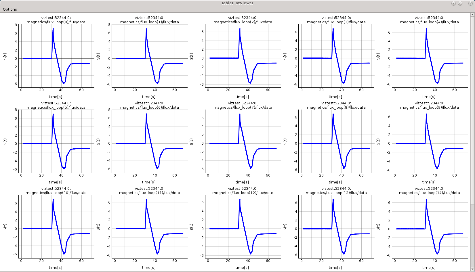
MultiPlot - Table Plot View Example.
2.4.7.1.1. Creating New View
To create a new Table Plot View, follow the next steps:
Create a selection of nodes, as described in section Plotting a selection of 1D arrays to figure.
- When finished with node selection, either:
right-click on any FLT_1D node or
click Node Selection menu on menubar of the main tree view window.
From the pop-up menu, navigate and select Plot selected nodes to
->
TablePlotView  -> New ->
This IMAS database or
All IMAS databases
-> New ->
This IMAS database or
All IMAS databases  or.
or.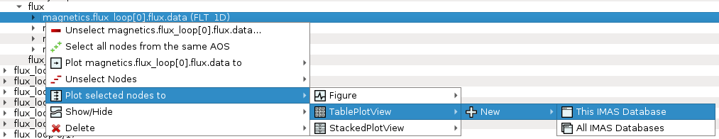
Plotting selection to a new figure using selection from the currently opened IDS database.
The Table Plot View window will then be created and shown.
Note
Each plot can be customized individually by right-clicking to the plot d display and selecting option Configure Plot.
Note
Scrolling down the Table Plot View window using the middle mouse button is disabled as the same button is used to interact with the plot display (zoom in and out). Scrolling can be done by clicking the scroll bar on the right and dragging it up and down.
2.4.7.1.2. Save MultiPlot Configuration
MultiPlot configuration (currently available only for Table Plot View feature) allows the user to save the MultiPlot session and load it later.
To create MultiPlot configuration, follow the next steps:
Create a selection of nodes, as described in section Plotting a selection of 1D arrays to figure.
Create a Table Plot View, as described in Table Plot View.
In Table Plot View menubar navigate to Options -> Save Plot Configuration
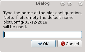
Save Plot Configuration Dialog Window.
Type configuration name in the text area.
Press OK.
Note
The configurations files are saved to $HOME/.imasviz folder.
2.4.7.1.3. Applying MultiPlot configuration to other IMAS database
To apply MultiPlot configuration to any IMAS database, follow the next steps:
Open IMAS database.
In Main Tree View Window menu navigate to Actions -> Apply Configuration. In the shown window switch to Apply Plot Configuration tab.
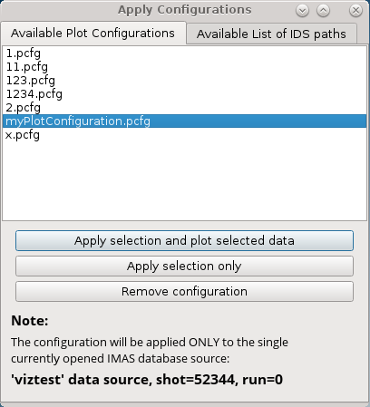
Apply Plot Configuration GUI Window.
Select the configuration from the list.
Press Apply selection and plot selected data.
The Table Plot View will be created using the data stored in the configuration file.
Note
Currently this feature will take all plot data from single (currently) opened IMAS database, event though MultiPlot configuration was made using plots from multiple IMAS databases at once. This feature is to be improved in the future.
Warning
The plots order depends on the order in which the data selection has been performed. First selected data will be the first plots in the Table Plot View window.
2.4.7.2. Stacked Plot View
Stacked Plot View allows the user to create a multiplot window by plotting every array from selection to its own plot display. The plot displays are arranged to resemble a stack layout, as shown in figure below. All plots displays always share the same X and Y range, even when using plot interaction features such as Zoom in/out, Pan Mode, Area Zoom Mode etc.
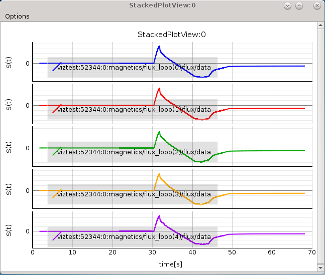
MultiPlot - Stacked Plot View Example.
2.4.7.2.1. Creating New View
To create a new Stacked Plot View, follow the next steps:
Create a selection of nodes, as described in section Plotting a selection of 1D arrays to figure.
- When finished with node selection, either:
right-click on any FLT_1D node or
click Node Selection menu on menubar of the main tree view window.
From the pop-up menu, navigate and select Plot selected nodes to
->
StackedPlotView  ->
New ->
This IMAS database or
All IMAS databases or.
->
New ->
This IMAS database or
All IMAS databases or.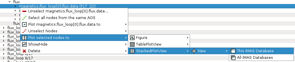
Plotting selection to a new figure using selection from the currently opened IDS database.
The Stacked Plot View window will then be shown.
Note
Each plot can be customized individually; right click on a node and select ‘Configure Plot’.