8. Conventions
8.1. Standard Machine Names
The following machine names are suggested:
aug
ftu
iter
jet
mast
tcv
tore_supra
west
8.2. Physics Conventions
The EU-IM-TF has agreed on a variety of conventions to facilitate the integration of the code modules across EFDA. In the following the most important conventions are explained in detail to remove confusion and avoid ambiguity. For more physical detail than that represented here see F Hinton and R Hazeltine, Rev Mod Phys 48 (1976) 239-308, or R Hazeltine and J Meiss, Plasma Confinement (Addison-Wesley, 1992).
8.2.1. Coordinate System
There are generally two choices for defining a right-handed coordinate system in a toroidal geometry with the following coordinates:
major radius R
vertical heights Z
toroidal angle \(\phi\)
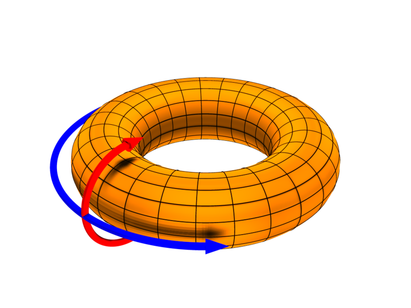
Remaining consistent with ITER, the EU-IM-TF has chosen to adopt the right-handed system
i.e. R is to the right, Z is upwards, and \(\phi\) points into the plane on the right-hand side of the torus (i.e. mathematically positive). Looking from above, the toroidal angle is counter-clockwise, i.e. mathematically positive.
The following figures demonstrate the orientation of the toroidal angle \(\phi\) and the poloidal angle \(\theta\):
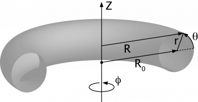
source:
http://www-fusion.ciemat.es/fusionwiki/index.php/Toroidal_coordinates
8.2.2. Representation of the Magnetic Field and Current
Generally, the magnetic field is described in terms of two scalar fields as it is divergence free. If the field is also axisymmetric then MHD equilibrium demands these are functions of each other. In the EU-IM-TF the relevant quantities are \(F_{{\rm dia}}\) and \(\Psi\) and the representation is
where the factor of \(2 \pi\) is to have \(\Psi\) one and the same with the poloidal flux in Webers (see below).
The current given by Ampere’s law is
The respective covariant toroidal components are useful forms:
where the latter is often expressed in terms of the “delta-star” operator, \(\Delta^* = R^2 \nabla \cdot R^{-2} \nabla\). These are not the toroidal field and current but the toroidal field and current multiplied by \(R\) respectively. The total plasma current \(I_p\) is the integral of \(J_{\phi} / R\) over the poloidal cross section (usually, but not always, over the closed flux surface region only).
8.2.3. Poloidal and Toroidal Fluxes
The toroidal flux \(\Phi\) is the integral of \(B_{\phi} / R\) over the region enclosed by the flux surface. Due to axisymmetry it is also a volume integral
All volume integrals are understood as integration over the region enclosed by the flux surface. They are therefore flux quantities (pure functions of \(\Psi\)). The units of \(\Phi\) are volt-seconds, or Webers (Wb).
The poloidal flux is \(\Psi\) due to the construction of \(\bf B\). The factor of \(2 \pi\) ensures this is not Wb per radian (the more usual quantity \(\psi\) used as a covariant toroidal component of the magnetic potential is in Wb/radian; the factor of \(2 \pi\) results from integration over one angular circuit). Note that the poloidal flux \(\Psi\) and its equivalent per radian \(\psi\) are often used equivalently in the literature.
8.2.4. Safety Factor
The magnetic pitch parameter is defined in terms of the flux components:
which is a flux quantity. This definition is the same as saying the magnetic pitch is given as the number of toroidal cycle a magnetic field line traverses per unit poloidal cycle. It is also called the local safety factor for MHD stability reasons (here, “local” means local to a given flux surface). Equivalent relations often seen depend on the definition of coordinates. These are given for straight field line coordinates, below.
8.2.5. Signs
With the above definition of the toroidal coordinate system and the magnetic field, the following sign relationships ensue (where increasing and decreasing refer to going from the magnetic axis to the separatrix on the outboard midplane):
\(B_{tor}\) |
\(I_{p}\) |
\(\Psi\) |
\(\Phi\) |
safety factor \(q\) |
|---|---|---|---|---|
positive |
positive |
decreasing |
increasing |
negative |
positive |
negative |
increasing |
increasing |
positive |
negative |
positive |
decreasing |
decreasing |
positive |
negative |
negative |
increasing |
decreasing |
negative |
8.2.6. COCOS - toroidal coordinate conventions
16 different fundamental coordinate conventions (COCOS) has been identified for toroidal systems. These are described by O. Sauter and S. Yu. Medvedev, Computer Phys. Commun. 184 (2013) 293.
The current EU-IM convention (described above) is number 13, while the ITER convention is 11.
8.2.6.1. Equilibrium COCOS transformation library and actor
A Fortran library has been developed for transforming the equilibrium cpo between different COCOS. The source is found in
https://gforge-next.eufus.eu/svn/numerical_tools/tags/COCOStransform_v1_1
and the actor is
https://gforge-next.eufus.eu/svn/kepleractors/tags/4.09a/imp12/COCOStransformequil.tar
(also available from: ~sauter/public/ACTORS/4.09a)
Inputs:
Equilibrium_in : input cpo
COCOS_in : COCOS of the input equilibrium (if the COCOS is not stored in Equilibrium_in)
COCOS_out : Requested COCOS for the Equilibrium_out
Ipsign_out : Requested sign for output Ip; -9 if just wants IP_in transformed to new equilibrium, +1 or -1 if a specific sign in output is desired
B0sign_out : Requested sign for output B0
Output:
Equilibrium_out : Output cpo
8.2.7. The Flux Surface Average
In general, the flux surface average is the operation which annihilates the magnetic derivative \({\bf B} \cdot \nabla\) and acts as an identity operator on any flux quantity. It can be proved that this results in a volume derivative of a volume integral (alternatively one starts with the latter property and then proves the former, as the above Ciemat reference does). The flux surface average of a scalar and divergence of a vector are given by
where \({\bf G} \cdot \nabla V\) is the contravariant volume component of the vector \({\bf G}\). It follows that the flux surface average is an angle average weighted by the volume element \(\sqrt{g}\)
for any choice of toroidal and poloidal angle as well as radial coordinates, where \(g\) is the determinant of the covariant metric tensor components in those coordinates. Note in general \(G\) is not an axisymmetric quantity so the integration is actually over both angles.
For more detail see the above references.
8.2.8. The Toroidal Flux Radius as the Radial Coordinate
The EU-IM-TF has decided to use the toroidal flux radius \(\rho_{{ \rm tor}}\) defined by
where \(B_0\) is the reference (vacuum) magnetic field value. Note that \(\rho_{{ \rm tor}}\) is a positive quantity which has units of meters. For several applications the volume radius \(\rho_{{ \rm vol}}\) is also used. It is a normalised radius going from 0 to 1 and is defined as
where LCFS refers to the last closed flux surface. Both should be defined in the equilibrium CPO (as well as \({ \tt volume} \equiv V\) itself).
8.2.9. Toroidal and Parallel Current
These are not equivalent, despite the often-seen experimental practice of considering them so. The toroidal current given in Amperes depends on some convention applied to \(J_{\phi}\) given above, which is not a flux quantity. The EU-IM-TF has decided on this definition of the toroidal current as a flux quantity:
This uses the contravariant toroidal component of \(\bf J\) which is a pure divergence
Hence the flux surface average invokes the often-used quantity \(\langle g^{\rho \rho}/R^2 \rangle\) in the form
Here, \(V'_\rho \equiv \partial V / \partial \rho_{{\rm tor}}\) explicitly using the toroidal flux radius as the radial coordinate.
The parallel current is different from this due to the finiteness of the poloidal current and magnetic field. Generally the correction is \(O( \epsilon^2 / q^2)\) which is usually a few percent (but not in a spherical tokamak). Using the representations for \(\bf B\) and \(\bf J\) given above we find
Since \(F_{{\rm dia}}\) is a flux quantity the flux surface average behaves as for \({\tt jphi}\) and we use a factor of \(B_0\) to provide the correct units, yielding
This form has been chosen due to the natural use of the flux surface average \(\langle{\bf J} \cdot{ \bf B} \rangle\) in neoclassical theory and the magnetic flux diffusion equation (see the Hinton and Hazeltine reference above).
8.2.10. Straight Field Line Coordinates
A variety of modules in the EU-IM-TF use straight field line coordinate systems to represent the closed flux surface region. To guarantee consistency with the definition of the poloidal flux and the magnetic field representation given above, a standard definition of the coordinate volume element follows. This is the same sense as the usage of the term “Jacobian” in the CPOs (note many papers use the inverse volume element as the “Jacobian” by contrast). Here, “straight field line coordinates” refers to the use of the right-handed coordinate system \((\Psi, \theta, \zeta)\) with the poloidal flux \(\Psi\), the straight field line angle \(\theta\), and the toroidal angle \(\zeta = - \phi\). Therefore, \(\theta\) has the same orientation as the poloidal angle \(\theta\) in toroidal coordinates, while the toroidal angle \(\zeta\) is in the opposite direction of \(\phi\). This is standard usage generally in terms of “flux coordinates” (see Hazeltine and Meiss, above).
Note here that while the toroidal angle is the geometric one in the orientation sense of flux coordinates, the poloidal angle is not geometric. This results from the demand that the field lines be straight in the coordinate plane \((\theta, \zeta)\). The definition of this property is given by the specification of the ratio of contravariant components of the magnetic field as a flux quantity, which is one and the same with the pitch parameter (“local safety factor”):
where the minus sign appears by consistency with the primary definition in terms of the flux components as given above. This represents a magnetic differential equation for the poloidal angle:
Due to the choice of “natural” coordinates (with \(\Psi\), not \(\rho_{{\rm tor}}\)) this relation is close to the definition of the volume element \(\sqrt{g}\) and, equivalently, the Jacobian \(J\)
Note the ordering of \({\bf \nabla} \Psi\) and \({\bf \nabla} \phi\).
The components of the magnetic field are then
With these relations the following relationship between the Jacobian and pitch parameter (“local safety factor”) holds
This is the quantity labelled \({\tt jacobian}\) in the equilibrium CPO.
8.2.11. Plasma Betas
Out of the many definitions of plasma betas, the EU-IM has agreed to adhere to the following definitions: Following Wesson (p. 116), the poloidal beta is defined as an integral over the poloidal cross section
where \(A = A (\Psi)\) is the poloidal cross section enclosed by the flux surface \(\Psi\), \(B_{\rm a} = \frac{ \mu_{0} I}{l}\) is the flux surface averaged poloidal magnetic field, \(I = I( \Psi )\) the toroidal plasma current inside the flux surface \(\Psi\) and \(l = \oint \rm{d} l\) the length of the poloidal perimeter of flux surface \(\Psi\). This definition yields a one-dimensional profile \(\beta_{\rm p} = \beta_{\rm p} ( \Psi )\) stored in profiles_1d%beta_pol in the equilibrium CPO. The overall poloidal beta \(\beta_{\rm p} (\Psi = \Psi_{\rm bd})\) is stored in global_param%beta_pol.
The toroidal beta is defined as
with \(B_{0}\) the vacuum magnetic field as stored in global_param%toroid_field%b0. The integral is carried out over the entire plasma volume and the result stored in global_param%beta_tor.
The normalized plasma beta is defined as
with \(I_{\rm p}\) the total plasma current (following Y.-S. Na et al., PPCF 44 (2002), 1285) and a is the minor radius. It is stored in global_param%beta_normal.
8.2.12. Internal Inductance
The definition of the internal inductance follows J.A. Romero et al., NF 50 (2010), 115002. The magnetic energy contained inside the flux surface \(\Psi\) is
where \(B_{\rm p}\) is the poloidal component of the magnetic field. The (unnormalized) internal inductance is then defined as
where \(I = I(\Psi)\) is the toroidal plasma current enclosed by the flux surface \(\Psi\). The normalized internal inductance, as stored in profiles_1d%li is defined as
with the surface averaged major radius
The overall internal inductance \(l_{\rm i} (\Psi = \Psi_{\rm bd})\) is stored in global_param%li.
8.2.13. Poloidal Angle Dimension in Equilibrium CPO
The following entries in the equilibrium CPO are defined along the poloidal dimension (as dim2 in the case of a flux surface equilibrium, i.e. radial coordinate psi in dim1 and poloidal angle in dim2):
coord_sys%jacobian(:,:)
coord_sys%g_11(:,:)
coord_sys%g_12(:,:)
coord_sys%g_13(:,:)
coord_sys%g_22(:,:)
coord_sys%g_23(:,:)
coord_sys%g_33(:,:)
profiles_2d%position
profiles_2d%grid
profiles_2d%psi_grid(:,:)
profiles_2d%jphi_grid(:,:)
profiles_2d%jpar_grid(:,:)
profiles_2d%br(:,:)
profiles_2d%bz(:,:)
profiles_2d%bphi(:,:)
The EU-IM-TF has decided not to repeat the first poloidal point (with poloidal angle \(\theta = 0\), which is identical to \(\theta = 2 \pi\). This option was chosen to facilitate Fourier transforms along the poloidal direction. To that purpose it is required that the dimension dim2 be equidistant in the poloidal angle \(\theta\) (going from \(\theta = 0\) to \(\theta = (ndim2-1)/ndim2*2 \pi\) where ndim2 is the number of poloidal grid points), whatever the choice of this angle is.
8.3. Numerical and computational conventions
8.3.1. Standardized Variable Types
To ensure that physics modules produce identical results on various computer architectures and to avoid issues with double precision versus single precision interfaces, the EU-IM-TF has agreed on a set of standardized variable types. It is recommended that these types be used throughout all EU-IM modules, but at least for the interface definitions. The Fortran90 module defining the type standards itm_types.f90 is hosted by the project itmshared . To check out the relevant files please do
svn checkout https://gforge-next.eufus.eu/svn/itmshared/trunk/src/itm_types target_dir
For Fortran90, the following standard types have been defined
INTEGER,  PARAMETER :: EU-IM_I1 = SELECTED_INT_KIND (2)        ! Integer*1
INTEGER,  PARAMETER :: EU-IM_I2 = SELECTED_INT_KIND (4)        ! Integer*2
INTEGER,  PARAMETER :: EU-IM_I4 = SELECTED_INT_KIND (9)        ! Integer*4
INTEGER,  PARAMETER :: EU-IM_I8 = SELECTED_INT_KIND (18)       ! Integer*8
INTEGER,  PARAMETER :: R4 = SELECTED_REAL_KIND (6, 37)   ! Real*4
INTEGER,  PARAMETER :: R8 = SELECTED_REAL_KIND (15, 300) ! Real*8
To implement these types in your code, please add the following line to your modules
use itm_types
(More information about the EU-IM libraries.)
8.3.2. Standardized Physical Constants
To avoid discrepancies in simulations from using different definitions of the physical constants, the EU-IM-TF has agreed upon a set of standardized physical constants (all in SI units except for temperatures) based on the NIST recommendations . It is recommended that these constant be used throughout all EU-IM modules. The Fortran90 module defining the standardized physical constants itm_constants.f90 is hosted by the project itmshared . To check out the relevant files please do
svn checkout https://gforge-next.eufus.eu/svn/itmshared/trunk/src/itm_constants target_dir
8.3.3. Invalid Data Base Entries
The EU-IM data base does not allow for setting data base entries directly to invalid in case they should not be set. Since the Universal Access Layer (UAL) always pulls out complete CPOs, i.e. complete data structures, of which not all fields may be filled, the problem arose of how to identify those fields which have not been filled. In the case of arrays, this is simply done by not associating the corresponding pointer. In the case of scalars, however, unique values for floats and integers had to be defined to identify empty fields. These values identify invalid data base entries and can be tested through comparison. The values for invalid data base entries in Fortran90 are defined below:
INTEGER,  PARAMETER :: itm_int_invalid = -999999999
REAL(R8), PARAMETER :: itm_r8_invalid = -9.0D40
They have been found to be safely out of any physical range for the affected fields such that no accidental confusion with real values may occur. The Fortran90 module defining these values itm_types.f90 is hosted by the project itmshared . To check out the relevant files please do
svn checkout https://gforge-next.eufus.eu/svn/itmshared/trunk/src/itm_types target_dir
The module also includes three functions of type boolean itm_is_valid_int4 , itm_is_valid_int8 , and itm_is_valid_real8 which are overloaded under the interface itm_is_valid to check whether a data base entry has been filled. Example:
if (itm_is_valid(equilibrium%global_param%i_plasma)) then
  write(*, *) 'Plasma current Ip = ', equilibrium%global_param%i_plasma
end if
8.3.4. Enumerated datatypes/Identifiers
This section concerns how to specify the origin of data in certain types of CPOs. The specification is performed using the datatype identifier. The following specifies the conventions of the allowed enumerated datatypes.
cocos_identifier.xml
coordinate_identifier.xml
coredelta_identifier.xml
coreneutral_identifier.xml
coresource_identifier.xml
coretransp_identifier.xml
distsource_identifier.xml
fast_particle_origin_identifier.xml
fast_thermal_filter_identifier.xml
fokker_planck_source_identifier.xml
pellet_shape_identifier.xml
species_reference_identifier.xml
wall_identifier.xml
wave_identifier.xml
8.3.4.1. Example: How to fill coresource/values/sourceid
When filling in an enumerated datatype, like coresource/values/sourceid, it is recomended to use the parameters and functions built into the fortran modules associated with each such datatype. These modules are available as part of the UAL package. As an examples we may include the coresource_identifier:
use coresource_identifier, only: fusion, get_type_name, get_type_description__ind
Here the value of the integer-parameter fusion is the Flag for fusion reactions in the coresource_identifier structure (i.e. fusion=5). Once we know the Flag we may get the Id using the function Id=get_type_name(Flag) and the Description using the function Description=get_type_description__ind(Flag). These function are available for every datatype.
Below you have an example of how to use these functions:
program coresource_example use euitm_schemas, only: type_coresource use
  coresource_identifier, only: fusion, get_type_name,
  get_type_description__ind use write_structures, only: open_write_file,
  write_cpo, close_write_file use deallocate_structures, only:
  deallocate_cpo implicit none

  type (type_coresource) :: coresource
  integer :: idx, i

  character*128 :: filename
  integer :: shot, run

  data filename / &
       & 'coresource.cpo' &
       & /

  allocate(coresource%values(1))
  allocate(coresource%values(1)%sourceid%id(1))
  allocate(coresource%values(1)%sourceid%description(1))
  coresource%values(1)%sourceid%flag = fusion
  coresource%values(1)%sourceid%id = get_type_name(fusion)
  coresource%values(1)%sourceid%description =
  get_type_description__ind(fusion)

  call open_write_file(1, filename)
  call write_cpo(coresource, 'coresource')
  call close_write_file

  call deallocate_cpo(coresource)

end program coresource_example
This example program, and similar examples for other enumerated datatypes, are available in:
https://gforge-next.eufus.eu/svn/itmshared/trunk/src/itm_constants/examples
8.3.5. Grid Types in Equilibrium CPO
Equilibria may be represented in a variety of different ways depending on which EU-IM module has calculated them and which module shall use them. To avoid ambiguity and to allow modules to check which type of equilibrium is stored in the equilibrium CPO, a unique grid identifier is stored in profiles_2d%grid_type. The grid identified currently consists of 4 strings (at 132 chars) with the following structure (array indices in Fortran notation):
Position |
Content |
|---|---|
grid_type(1) |
integer identifier for grid type |
grid_type(2) |
string identifier for grid type |
grid_type(3) |
integer identifier for poloidal angle |
grid_type(4) |
string identifier for poloidal angle |
8.3.5.1. Grid Type Identifier
The currently allowed values (integer and string) for the identifier of the grid type are listed below:
Integer Values |
String Value |
Description |
|---|---|---|
1 |
rectangular |
Regular grid in \((R,Z)\). ‘EFIT-like grid’ |
2 |
inverse |
Regular grid in \(\Psi,\theta\). ‘flux surface grid’. |
3 |
irregular |
Irregular grid. All fields in
profiles_2d are given as (ndim1,
1)
degenerate 2D matrices, i.e.
as lists of vertices (for
triangles or quadrilaterals).
|
8.3.5.1.1. Poloidal Angle Identifier
The currently allowed values (integer and string) for the identifier of the poloidal angle are listed below:
Integer Values |
String Value |
Description |
|---|---|---|
1 |
straight field line |
straight field line angle \(\theta\) as defined in Straight Field Line Coordinates |
2 |
equal arc |
Poloidal angle \(\theta\) defined by equal arc lengths along flux surfaces |
3 |
polar |
Poloidal angle \(\theta\) in toroidal coordinates as defined in Coordinate System |
8.3.6. Standardized EU-EU-IM Plasma Bundle
The EU-IM has agreed on a standardized way to bundle CPOs and control parameters inside KEPLER.
Field names |
Type |
Description |
||
|---|---|---|---|---|
time |
real |
The synthetic time of the simulation,
or for time-dependent workflows; the
end of the present time step. For
example, consider a time dependent
workflows, where physics quantities
are update one after the other. Thus,
while the physics quantities are
updated the various fields below
(e.g. the CPOs) may be describe at
different time points. In such
workflows the this “time”-field
describe the time at the end of the
present time step. Units: (s)
|
||
CONTROL |
tau |
real |
time-step (s) |
|
tau_out |
real |
time interval for saving output (s) |
||
ETS |
amix |
real |
mixing factor |
|
amix_tr |
real |
mixing factor for profiles |
||
sigma_source |
integer |
option for origin of plasma electrical
conductivity: 0: plasma collisions;
1: transport module; 2: source module
|
||
solver_type |
integer |
choice of numerical solver |
||
conv_rec |
real |
required fractional convergence |
||
CPOS |
MHD |
equilibrium |
cpo |
see type and fortran descriptions |
toroidfield |
cpo |
see type and fortran descriptions |
||
mhd |
cpo |
see type and fortran descriptions |
||
sawteeth |
cpo |
see type and fortran descriptions |
||
CORE |
coreprof |
cpo |
see type and fortran descriptions |
|
coretransp |
cpo |
see type and fortran descriptions |
||
coresource |
cpo |
see type and fortran descriptions |
||
coreimpur |
cpo |
see type and fortran descriptions |
||
coreneutral |
cpo |
see type and fortran descriptions |
||
corefast |
cpo |
see type and fortran descriptions |
||
coredelta |
cpo |
see type and fortran descriptions |
||
compositionc |
cpo |
see type and fortran descriptions |
||
neoclassic |
cpo |
see type and fortran descriptions |
||
EDGE |
edge |
cpo |
see type and fortran descriptions |
|
HCD |
waves |
cpo |
see type and fortran descriptions |
|
distsource |
cpo |
see type and fortran descriptions |
||
distribution |
cpo |
see type and fortran descriptions |
||
MACH |
vessel |
cpo |
see type and fortran descriptions |
|
wall |
cpo |
see type and fortran descriptions |
||
nbi |
cpo |
see type and fortran descriptions |
||
antennas |
cpo |
see type and fortran descriptions |
||
ironmodel |
cpo |
see type and fortran descriptions |
||
pfsystems |
cpo |
see type and fortran descriptions |
||
DIAG |
fusiondiag |
cpo |
see type and fortran descriptions |
|
scenario |
cpo |
see type and fortran descriptions |
||
EVENTS |
pellets |
cpo |
see type and fortran descriptions |
|