3. European Transport Simulator (ETS)

3.1. ETS Documentation

This page contains useful information on the European Transport Simulator (ETS) including documentation, description of the pre and post-processing tools used with ETS as well as instructions on how to use ETS and tools on the EUROfusion Gateway.

3.1.1. Configuration of the ETS-5 workflow in Kepler

ETS-5 uses CPO for actor integration in Kepler and as input data to the workflow. This means that the user environment needs to be set up as ITM environment.

To do so login on the EUROfusion Gateway and type the following commands:

module purge
module load cineca
module load itmenv/ETS_4.10b.10_v5.7.0
source $ITMSCRIPTDIR/ITMv2.sh jet
export ITM_KEPLER_DIR=$ITMWORK/my_keplers
export _JAVA_OPTIONS="-Xss20m -Xms4g -Xmx8g -Dsun.java2d.xrender=false"

The command ‘module load itmenv/ETS…’ loads the itmenv environment and in particular in the case above the ETS / Kepler version 5.7.0 To load a different version just change the number e.g. v5.5.0

The $ITMSCRIPTDIR/ITMv2.sh JET command will set up your local database folder to ‘JET’. This means that any simulation done with ETS will be saved in the JET folder (even if you are simulating TCV!!). If you would like to simulate any other Tokamak, type again the command and change JET with e.g. AUG.

The remaining commands are JAVA options for running Kepler and setting of MPI useful for running parallel actors.

If it is the first time you run ETS then you will need to install your first ‘dressed’ Kepler version which corresponds to Kepler with all the WPCD actors embedded in it.

This can be done by executing the following command

install_kepler.sh ets_v570 trunk/ETS_4.10b.10_v5.7.0/central "dressed central kepler v5.7.0"
switch_to_kepler.sh ets_v570

For loading the Workflow+tools (import data, postprocessing):

svn co https://gforge-next.eufus.eu/svn/keplerworkflows/tags/ETS_4.10b.10_v5.7.0

The above command requires enabled access to GFORGE (if you are a ‘simple’ user you might need to apply for access to GFORGE). Typing the command above will check out and store the ETS_worflow.xml and useful python scripts in the directory from where it is issued.

Plotting routines such as kplots can be found under

>cd $KEPLER

You are now ready to start ETS!!

The latest version of ETS-5 is v5.5.0 (09/12/2019)

To launch Kepler and load the ETS-5 workflow just type

>kepler.sh

or if you like to see the the log messages printed on the scree while ETS runs

>kepler.sh -nolog

Once the Kepler canvas opens, chose the option ‘load workflow’ from the File menu and select the workflow you would like to load. The recommendation is to use the ETS workflow released with the version release procedure and then upload your parameter settings via the parameter file. See the option - running ETS with autoGui

A video showing how to run and set up ETS-5 can be viewed here

https://www.youtube.com/watch?v=dv427_XOFf4&t=87s

3.1.2. ETS releases

ETS release 5.5.0 is installed on the Gateway.

Quick installation instructions (to update your environment) are available here (password protected areas):

https://portal.eufus.eu/twiki/bin/view/Main/Installation_of_latest_kepler_release

Detailed instructions are available here:

https://portal.eufus.eu/twiki/bin/view/Main/User_Guide_accessing_JET_data

List of modifications (as compared to the previous release) is available here:

https://portal.eufus.eu/twiki/bin/view/Main/Updates_550

3.2. ETS workflows in KEPLER

The ETS workflow is used for 1-D transport simulation of a tokamak core plasma.

ETS workflows in KEPLER:

• use actors and composite actors from the WPCD / IMAS fusion library

• complex, but clearly structured workflow, which offers user friendly interface for configuring the simulation

• allow for easy modifications (connecting new modules, or reconnecting parts of the workflow) through an easy graphical interface

• provide users with all updates through the version control system

• still in active development tool (ETS-6)

Starting the workflow: If you have the workflow already installed, there are several ways to execute it:

• For execution via kepler GUI:

>kepler.sh workflow_path/workflow_name.xml

• for executution via autoGui

>autoGui

once the GUI opens select load workflow after which a parameter file can be loaded. You can create a parameter file by loading the standard workflow released with the Kepler version and then chosing the option from the top menu ‘save parameter file’. The use of autoGui is strongly recommanded as worklows are large xml files while parameter files are small and do not take all your disk space. Moreover parameter files can be loaded in any version of ETS-5 by opening the standard workflow included in the release.

3.2.1. Configuring the ETS run

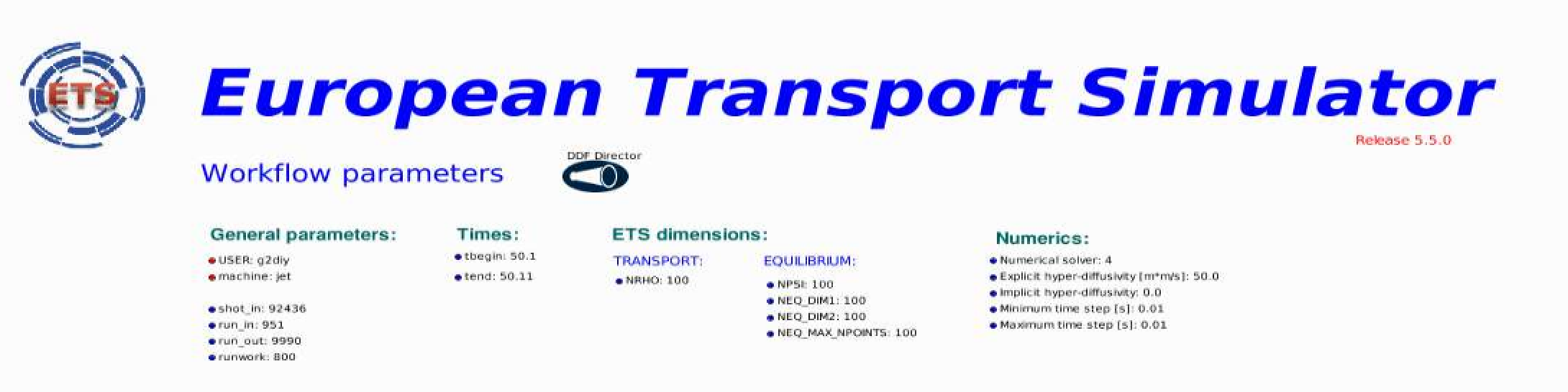
3.2.1.1. Workflow parameters

3.2.1.1.1. General Parameters

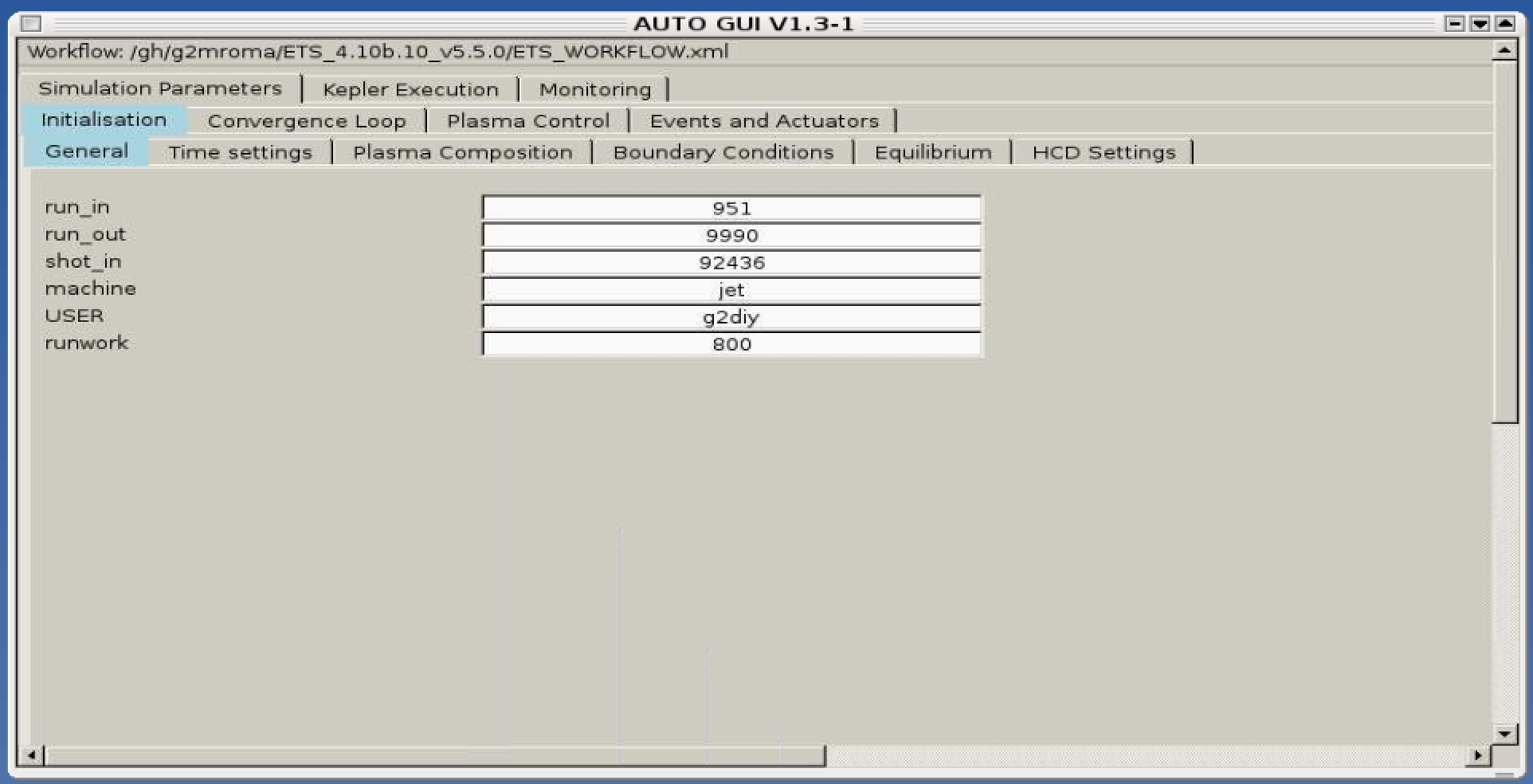
• USER - your userid

• MACHINE - machine name (database name) for which comutations are done

• SHOT_IN - input shot number

• RUN_IN - input run number

• RUN_OUT - output run number

• RUNWORK - work directory number (typically 800)

3.2.1.1.2. Time resolution

Start and End time:

• TBEGIN - Computations start time

• TEND - Computations end time

3.2.1.1.3. Transport

• NRHO - number of radial points for transport equations

3.2.1.1.4. Equilibrium

• NPSI - number of points for equilibrium 1-D arrays

• NEQ_DIM1 - number of points for equilibrium 2-D arrays, first index

• NEQ_DIM2 - number of points for equilibrium 2-D arrays, second index

• NEQ_MAX_NPOINTS - maximum number of points for equilibrium boundary

3.2.1.1.5. Numerics

• NUMERICAL_SOLVER - choice of the numerics solving transport equations (RECOMENDED SELECTION: 3 or 4)

• EXPLICIT HYPER DIFFUSIVITY - Constant diffusivity used in the stabilization scheme needed to deal with stiff transport models

• IMPLICIT HYPER DIFFUSIVITY - Same as above used in the implicit part of the solver

• MINIMUM TIME STEP - Minimum time step allowed in the transport solver

• MAXIMUM TIME STEP - Maximum time step allowed in the transport solver

3.2.1.1.6. Equilibrium

• NPSI - number of points for equilibrium 1-D arrays

• NEQ_DIM1 - number of points for equilibrium 2-D arrays, first index

• NEQ_DIM2 - number of points for equilibrium 2-D arrays, second index

• NEQ_MAX_NPOINTS - maximum number of points for equilibrium boundary

Time step:

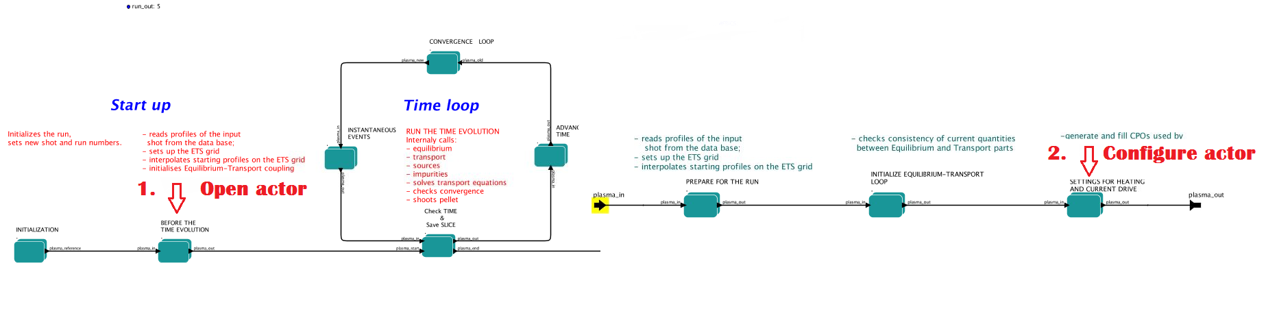
• right click on the box BEFORE THE TIME EVOLUTION

• select Configure actor

• TAU :specify value of the time step in [s]

• TAU_OUT : specify value of the output time interval in [s]

• Commit

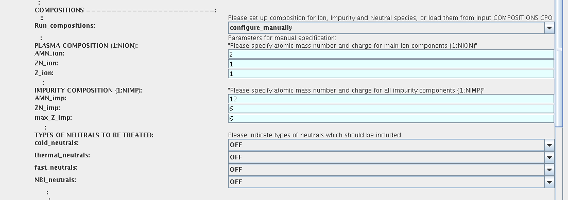
3.2.1.2. Ion, Impurity and Neutral Composition

Before starting the run you need to define types of main ions, impurity (optional) and neutrals (optional) to be included in simulations.

To define plasma composition:

• right click on the box BEFORE THE TIME EVOLUTION

• select Configure actor

• choose one of modes for setting Run_compositions

  • from_input_CPO - will pick up the COMPOSITIONS structure of the COREPROF CPO saved to the input shot;

  • configure_manually - will force the composition from the values specified below

• specify values of atomic mass (AMN_ion), nuclear charge ( ZN_ion ) and charge ( Z_ion , from the first ion to the last [1:NION] , separated by commas

• (optional) specify values of atomic mass ( AMN_imp ), nuclear charge ( ZN_imp ) and maximal ionization state ( max_Z_imp ) for impurity ions, from the first to the last [1:NIMP] , separated by commas

• (optional)for neutrals activate, by switchen them to ON, the types which shall be followed by neutral solver

• press Commit

3.2.1.3. Equations to be solved and boundary conditions

3.2.1.3.1. Main Plasma

Before starting the run you need to select the type and value of the boundary conditions for all equations. Please note that the value should correspond to the type. All equations allow for following types of boundary conditions:

• OFF - equation is not solved, initial profiles will be kept for whole run

• value - edge value should be specified

• gradient - edge gradient should be specified

• scale_length - edge scale length should be specified

• generic - generic form: a1*y´ + a2*y = a3 of the boundary condition is assumed, 3 coefficients (a1, a2, a3) should be provided

• value_from_input_CPO - equation is solved, edge value evolution will be red from input shot

• profile_from_input_CPO - equation is not solved, profile evolution will be red from input shot

The particular equation will be activated if the boundary condition type for it is other than OFF

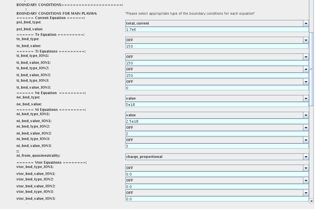
To set up boundary conditions:

• right click on the box BEFORE THE TIME EVOLUTION

• select Configure actor

• select appropriate boundary condition for each equation

• specify values for boundary conditions corresponding to the type and to the ion component

• Commit

The workflow will not allow the user all particle components (ions[1:NION]+electrons) to be run predictively. At least one of them shall be set to OFF (this component will be computed from quasi-neutrality condition).

!!! If electron density is solved, all ions with ni_bnd_type=OFF will be computed from the quasineutrality condition and scaled proportional to specified ni_bnd_value or inversely proportional to their charge, charge_proportional. This is defined by option: ni_from_quasineutrality.

3.2.1.3.2. Impurity

You can set up the boundary conditions for impurity ions in a similar way as for main ions. !!! Note, that at the moment only types: OFF; value and value_from_input_CPO are accepter by impurity solver.

To set up boundary conditions:

• right click on the box BEFORE THE TIME EVOLUTION

• select Configure actor

• select appropriate boundary condition for each impurity species ( OFF-equation is not solved)

• specify values for boundary density of each impurity component [1:MAX_Z_IMP], separated by commas

• Commit

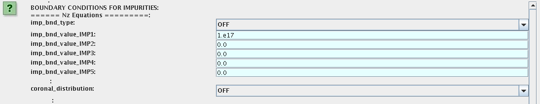
Interface for impurity boundary condition has additional option, coronal_distribution, that allow to preset the edge values or entire profiles of individual ionization states from coronal distribution. In tis case only single value is required to be specified for each impurity boundary value. The options are:

• OFF - the boundary values for impurity densities will be as they are specified above;

• boundary_conditions - the boundary densities will be renormalized with corona, using the first element from above as a total density

• boundary_conditions_and_profiles - the boundary densities and starting profiles will be renormalized with corona, using the first element from above as a total density

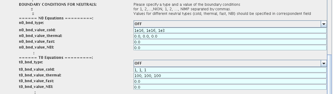
3.2.1.3.3. Neutrals

Note, that ALL values should be specified in the order: {1, 2, 3 …NION, 1, 2, 3, …NIMP}

To set up boundary conditions:

• right click on the box BEFORE THE TIME EVOLUTION

• select Configure actor

• select appropriate boundary condition for each neutral species (OFF-equation is not solved)

• specify values for boundary density and temperature of each neutral component [1, 2, 3 …NION, 1, 2, 3, …NIMP], separated by commas

• Commit

3.2.1.3.4. Input profiles interpolation

You are going to start the ETS run from some input shot, which might contain some conflicting rho grids saved to different CPOs. Thus there is a choice for the user to decide on the grid on which the starting profiles should be load by the worflow,

Interpolation_of_input_profiles.

To define the interpolation grid select:

• on_RHO_TOR_grid - interpolate input profiles based on the grid specyfied in [m];

• on_RHO_TOR_NORM_grid - interpolate input profiles based on normalised rho grid [0:1]

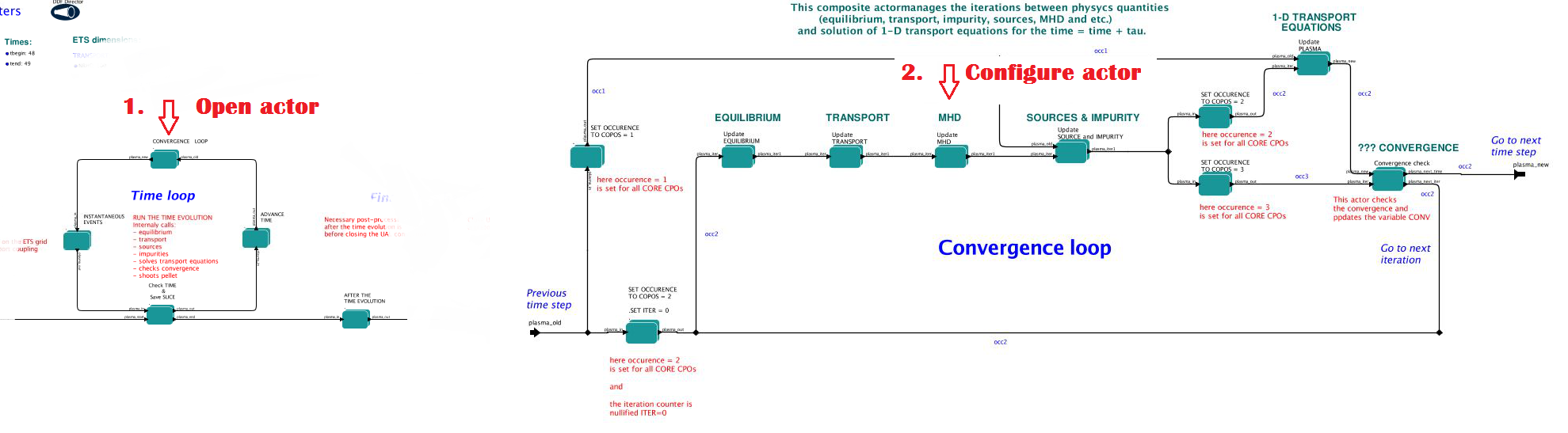
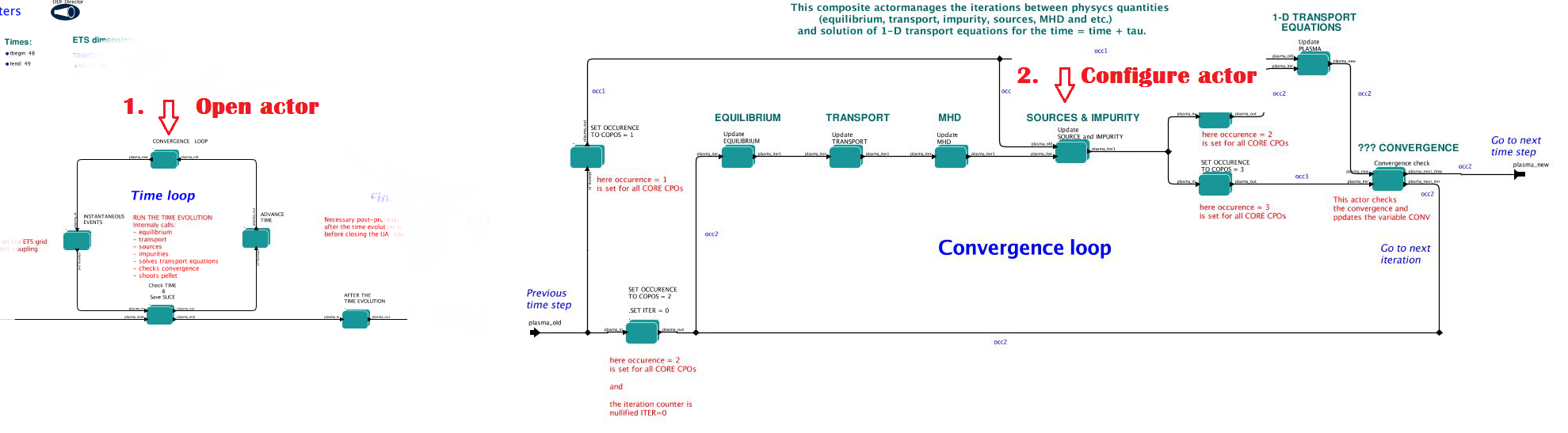
3.2.1.4. Convergence loop

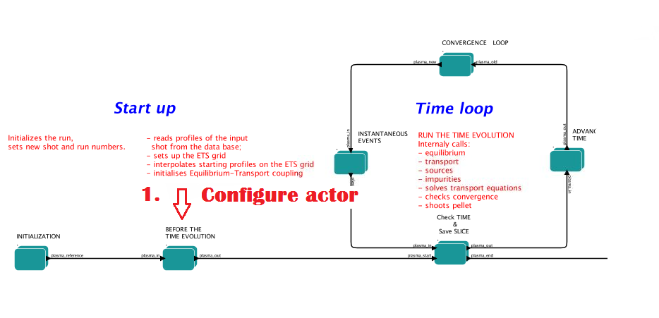
ETS updates input from different physics actors in a sequence, which is finished by solving the transport equations. Ther are possible none-linear couplings between different parts of the system. These nonelinearities are treated by the ETS using iterations. The decision to step in time is made by the ETS based on the criteria that the maximum relative deviation of main plasma profiles is lower than some predefined tolerance. There is a number of settings and switches in the ETS that are used by the iterative scheme. To edit them do:

• right click on the box CONVERGENCE LOOP

• select Configure actor to edit settings

• choose your settings

• Commit

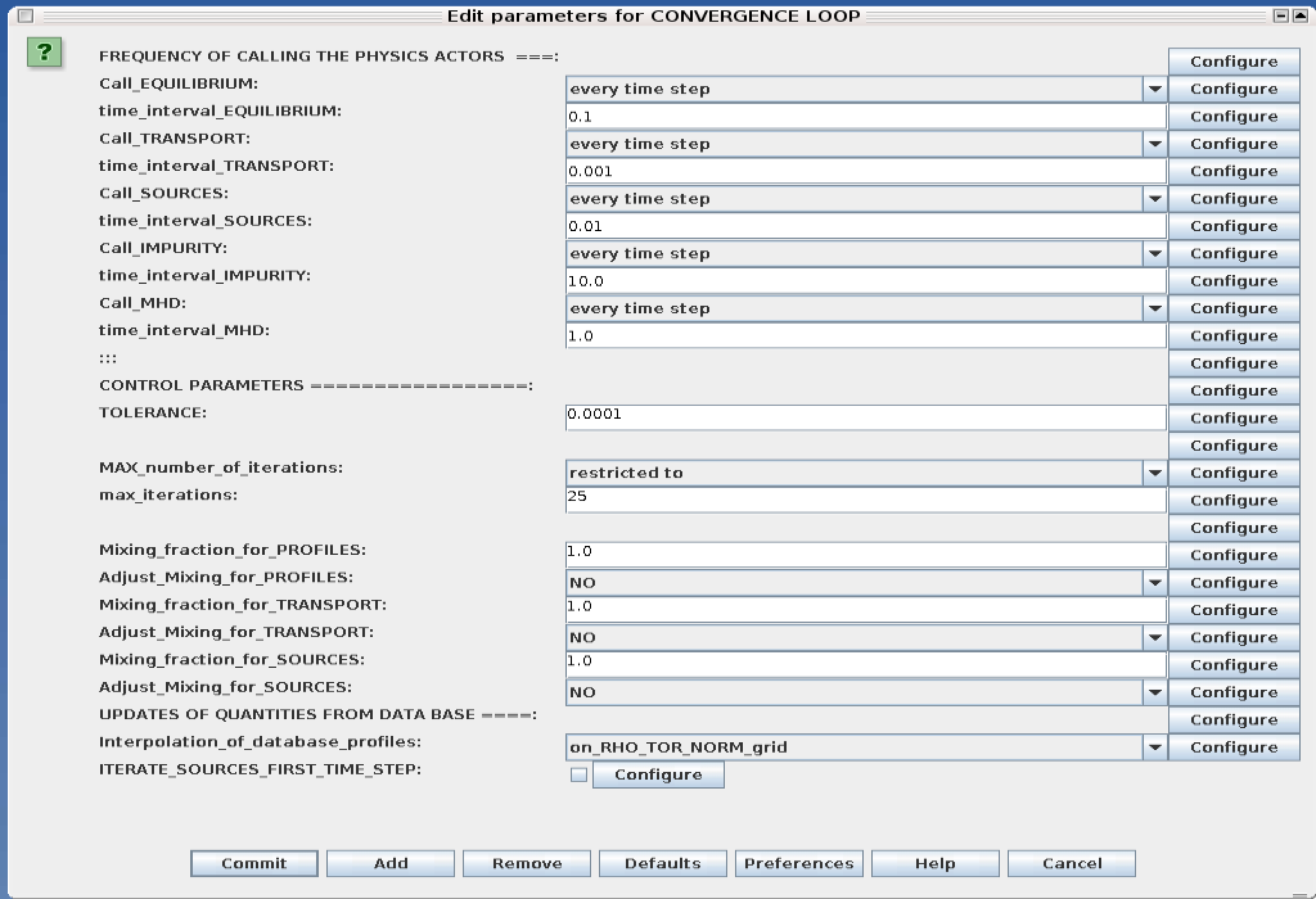
Switches in the field FREQUENCY OF CALLING THE PHYSICS ACTORS define how many times the actors of a certain cathegory (equilibrium, transport, etc.) should be called.

Switches and parameters in the field CONTROL PARAMETERS define how iterations are done

• Tolerance - defines the maximum relative error of profiles change compared to previous iteration. If it is achieved the time steping is done.

For highly none-linear case the required precision can be achieved faster by the iterative scheme if only fraction of the new solution is mixed to the previous state. The following scheme is adopted by the ets to reduce none-linearities in profiles, transport coefficients and sources:

Y = (Amix * Y+) + ((1-Amix)*Y-)

where Amix is the mixing fraction You can activate the mixing of profiles, transport coefficient and sources by selecting the corresponding Mixing_fraction_… to be between [0:1] You also can activate the authomatic ajustment of this fraction by selecting: Ajust_Mixing_for_… to YES

3.2.1.5. Equilibrium

3.2.1.5.1. Initialization Settings

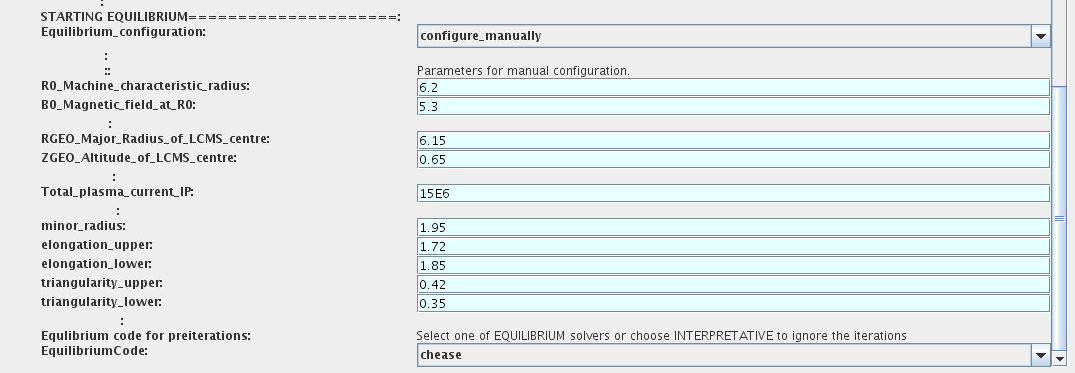
Before starting the run you need to set up your initial equlibrium. There are several options to do it: if your input shot contains the consistent equilibrium with all necessary parameters - you can start immediately from it; if your input shot contains the equilibrium but it is not consistent or some parameters are missing you can check it automatically; if your input equilibrium is corrupt or not present - you can define the starting equlinbrium by tree moment description. To select your starting equilibrium please do:

• right click on the box BEFORE THE TIME EVOLUTION

• select Configure actor to edit settings

• Select your settings or specify values

• Commit

SETTINGS:

• Equilibrium_configuration - select configure_manually if you like to specify configuration below; select from_input_CPO if all quantities should be picked up from the input CPO

• R0_Machine_characteristic_radius - Characteristic radius of the machine, here B0 is measured [m]

• B0_Magnetic_field_at_R0 - Magnetic field measured at the position R0 [T]

• RGEO_Major_Radius_of_LCMS_centre - R coordinate of the geometrical centre of the LCMS [m]

• ZGEO_Altitude_of_LCMS_centre - Z coordinate of the geometrical centre of the LCMS [m]

• Total_plasma_current_IP - plasma current within the LCMS [A]

• Minor_radius - minor radius of the LCMS [m]

• Elongation - elongation of the LCMS [-]

• Triangularity_upper - upper triangularity of the LCMS [-]

• Triangularity_lower - lower triangularity of the LCMS [-]

• Equilibrium code - select one of available equilibrium solvers to check the consistency between starting equilibrium and current profile; use INTERPRETATIVE if you trust your input data (in this case the check will be ignorred).

Please note, that different equilibrium solvers might require slightly different input. Thus it is a user responsibility to check that the information inside input shot/run is enough to run selected equilibrium solver.

3.2.1.5.2. Run Settings

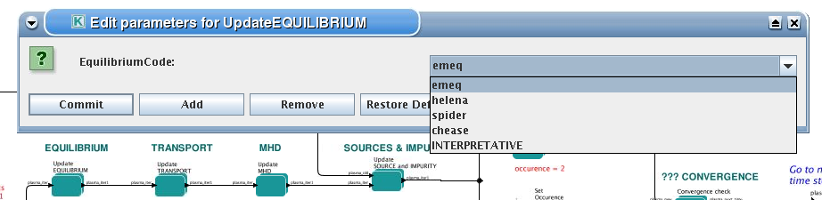
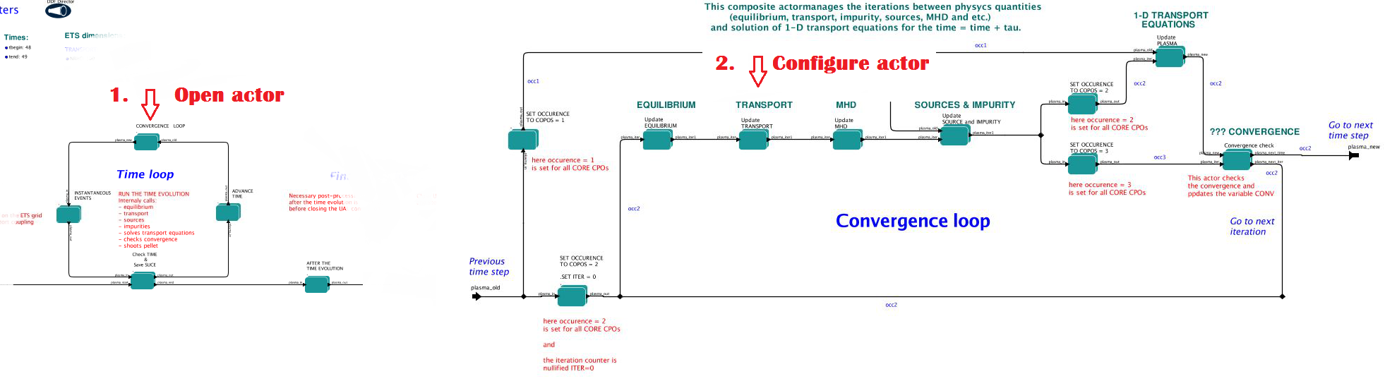
There are several equilibrium solvers connected to the ETS. You can select the one of them.Therefore please do:

• right click on the box CONVERGENCE LOOP

• select Open actor

• right click on the box EQUILIBRIUM

• select Configure actor to edit settings

• choose your equilibrium solver

• Commit

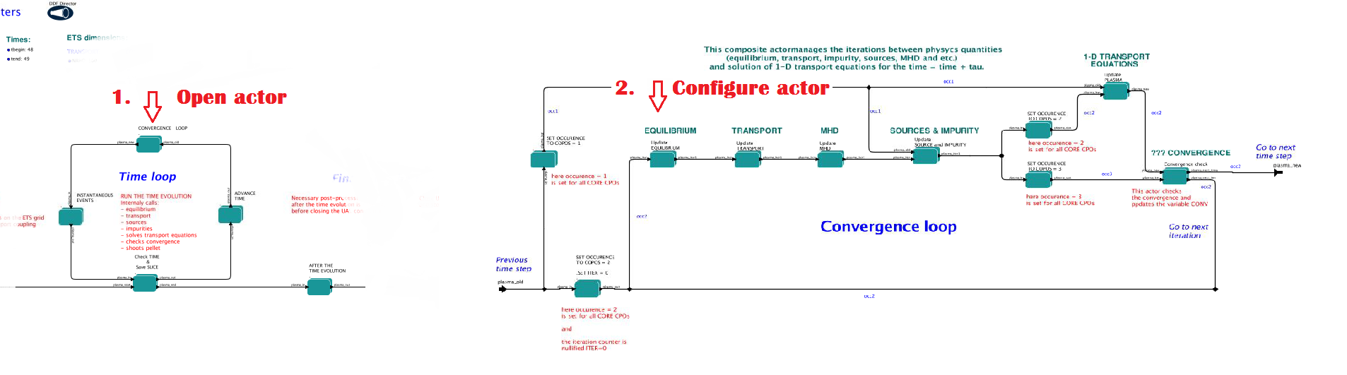
INTERPRETATIVE means that the ETS will not update the equilibrium, instead it will be using the initial equilibrium.

Please note, that it is better to select the same code as you used for pre-iterrations. Because outputs of different equilibrium solver are not necessary done with the same resolution. Therefore the routine saving the information to the data base might brake due to uncompatible sizes of some signals.

3.2.1.6. Transport

The settings for TRANSPORT can be done inside the CONVERGENCE LOOP composite actor. Therefore please do:

• right click on the box CONVERGENCE LOOP

• select Open actor

• right click on the box TRANSPORT

• select Configure actor to edit settings

• choose your settings

• press Commit

3.2.1.6.1. Transport models

ETS constructs the total transport coefficients from the combination of Anomalous transport (model choice), Neoclassical transport (model choice), Database transport (transport coefficients be saved to the input shot) and Background transport (Transport coefficients defined through the GUI interface)

D_tot = D_DB*M_DB + D_AN*M_AN + D_NC*M_NC + D_BG*M_BG

You should choose from the list of evailable models in each cathegory or switch it OFF

Individual multipliers for all channels shall be specified on the lower level through the code parameters of Transport Combiner

3.2.1.6.2. Background transport

You can add the constant background level for each coefficient (ion and impurity coefficients are expected to be the strings of [1:NION] and [1:NIMP] elements respectively, separated by commas)

3.2.1.6.3. Edge transport barrier

In this section you can artificially supress the transport outside of specified RHO_TOR_NORM_ETB. Total transport coefficients for all transport channels (ne, ni, nz, Te, Ti,…) will be reduced to constant values specified below (ion and impurity coefficients are expected to be the strings [1:NION] and [1:NIMP] respectively)

3.2.1.6.4. Total transport coefficients

The fine tuning of of transport coefficients can be done through editing the XML code parameters of the transport combiner actor:

• In Outline browse for transportcombiner

• select Configure actor

• click Edit Code Parameters

• • If you select OFF contributions from all transport models to this channel will be nullified;

  • If you select Multipliers_for_contributions_from the transport channel will be activated, and the total transport coefficient will be combined from active tranport models. You gust need to specify multiplier against each channel;

  • For convective velocity there is an additional option V_over_D_ratio_for_contributions_from. With this option selected the combiner will ignore the convective components provided by transport models. The convective velocity will be determined from the diffusion coefficient by applying fixed V/D ratio ( for inward pinch the values should be negative! ).

• Save and exit

• Commit

3.2.1.7. MHD

The settings for MHD type of events can be done inside the CONVERGENCE LOOP composite actor. Therefore please do:

• right click on the box CONVERGENCE LOOP

• select Open actor

• right click on the box MHD

• select Configure actor to edit settings

• choose your settings

• Commit

At the moment ETS allows only for NTM to be activated.

User can ajust the following NTM settings:

• NTM – ON means that ETS will add the NTM driven transport to the total transport coefficient; OFF -ignored

• NTMTransportMultiplier – the transport contrinution from NTM will be multiplied with this value

• Onset_NTM_time - activation time for the NTM mode

• Onset_NTM_width - starting width of the mode

• m_NTM_poloidal_number

• n_NTM_toroidal_number

• NTM_phase

• NTM_frequency

3.2.1.8. Sources and impurity

The settings for SOURCES AND IMPURITY can be done inside the CONVERGENCE LOOP composite actor. Therefore please do:

• right click on the box CONVERGENCE LOOP

• select Open actor

• right click on the box SOURCES AND IMPURITY

• select Configure actor to edit settings

• choose your settings

• Commit

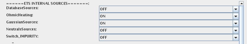
3.2.1.8.1. Analytical & Impurity sources

There is a number of sources developed by WPCD, which are actors or internal routines of the transport solver. You can activate them by selecting ON / OFF in front of corresponding source:

• Database Sources – ON - ETS will pick up the evolution of source profiles saved to your input shot/run; OFF -ignored

• Ohmic Heating – ON - ETS will compute Ohmic heating internaly; OFF -ignored

• Gaussian Sources – ON - ETS will add sources from the Gaussian source actor (you can configure heat and particle deposition profiles by editing the code parameters of the actor); OFF -ignored

• Neutral Sources – ON - Fluid neutrals will be solved according to the boundary conditions specified on ¨Before_time_evolution¨ composite actor interface; OFF -ignored

• Switch_IMPURITY – ON - Impurity density and radiative sources will be computed; OFF -ignored; INTERPRETATIVE – profiles of impurity density will be read from input shot/run

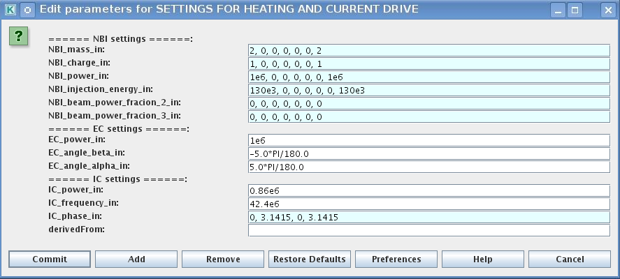
3.2.1.8.2. HCD sources

There is a number of sources developed by WPCD, that are incorporated by the ETS workflow.

For the HCD sources please activate the type of heating source, by ticking the box in front of it, and select the code to simulate it.

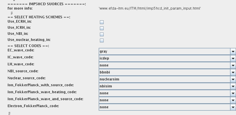
You also need to configure initial HCD settings. Therefore please:

• right click on the box BEFORE THE TIME EVOLUTION

• select Open Actor

• right click on the box SETTINGS FOR HEATING AND CURRENT DRIVE

• select Configure actor

• edit the stettings

• Commit

Please note that settings for NBI are done independent for each PINI. Therefore, for NBI settings, please insert the values separated by commas. The number of the element in the array corresponds to the number of activated PINI. Maximum accepted number of PINIs = 16.

3.2.1.8.3. Power control

You also can activate the power control for the IMP5HCD sources.

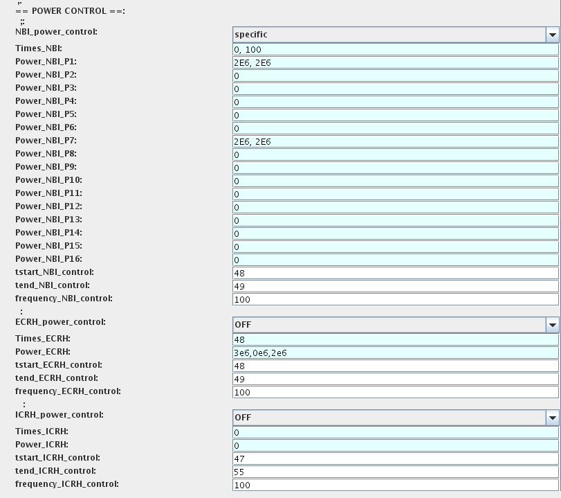
If the POWER_CONTROL is not OFF, there are two modes of operation: specific and frequency

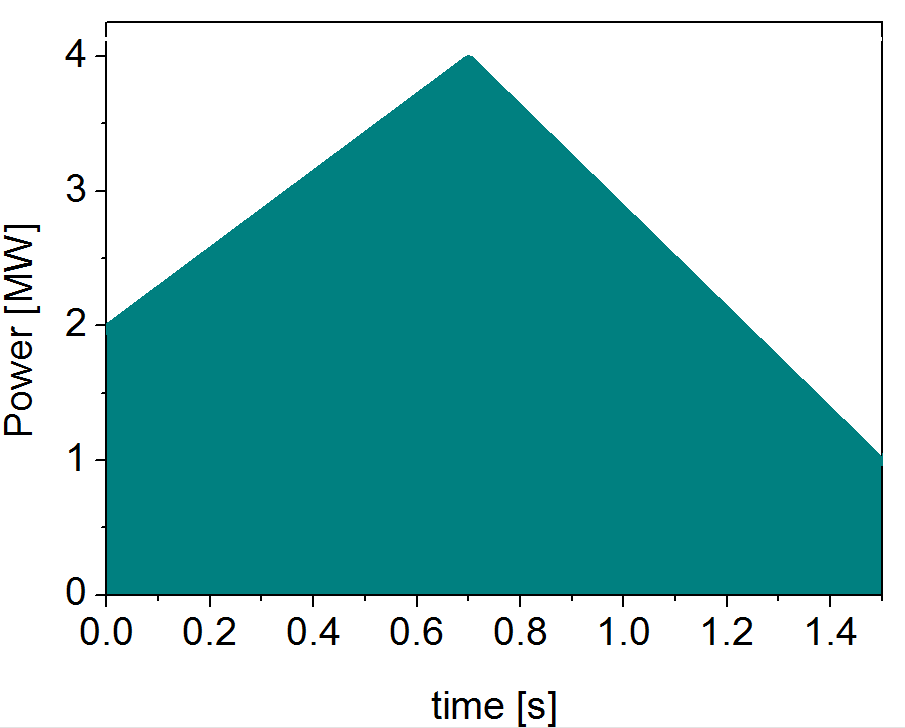
For specific you should specify the time sequence separated by commas and the corresponding power sequence (where first power level corresponds to the first time, second to second and etc.). Linear interpolation will be done between the sequence points. For example: if you give the power sequence = 2e6,4e6,1e6 and times = 0.0, 0.7, 1.5 (s) the delivered power would be:

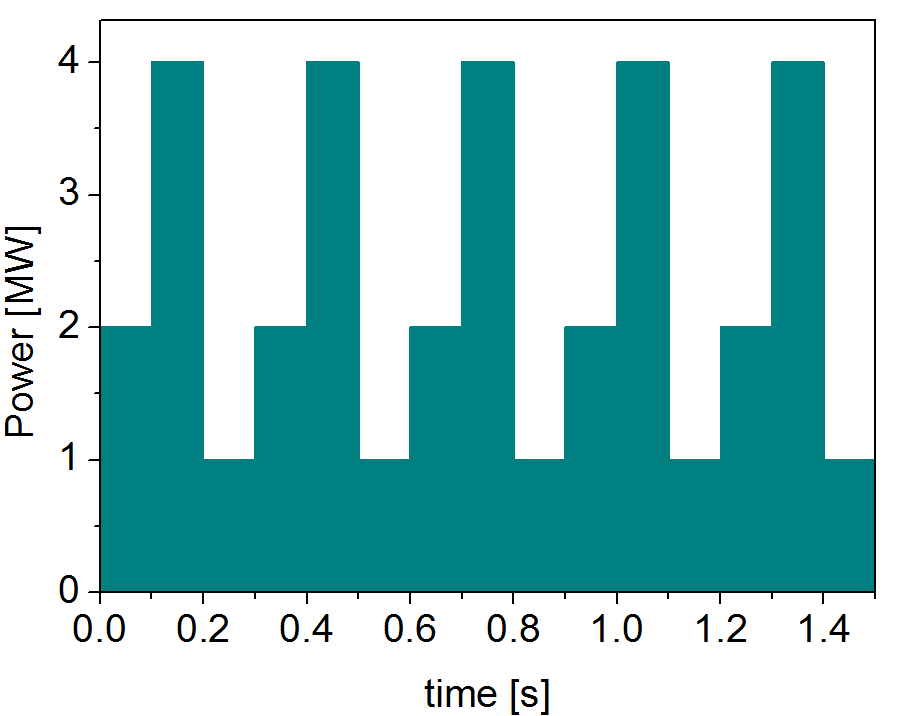
For frequency you should specify the power levels sequence separated by commas, start and end time of the power control and the frequency of switching between these levels. For example: if you give the power sequence = 2e6,4e6,1e6 and frequency = 10 (Hz) tstart = 0.0 (s) tend = 1.5 (s) the delivered power would be:

3.2.1.8.4. Total power

Profiles of the total source for each channel are obtained from the the individual contributions (Data Base, Gaussian, Neutrals, Impurity and HCD) as a summ of all activated sources multiplied with coefficients specified on the interface of the composite actor.

S_tot = S_DS*DSM + S_GS*GSM + S_Neu*NeuSM + S_IMP*IMPSM + S_HCD*HCDSM

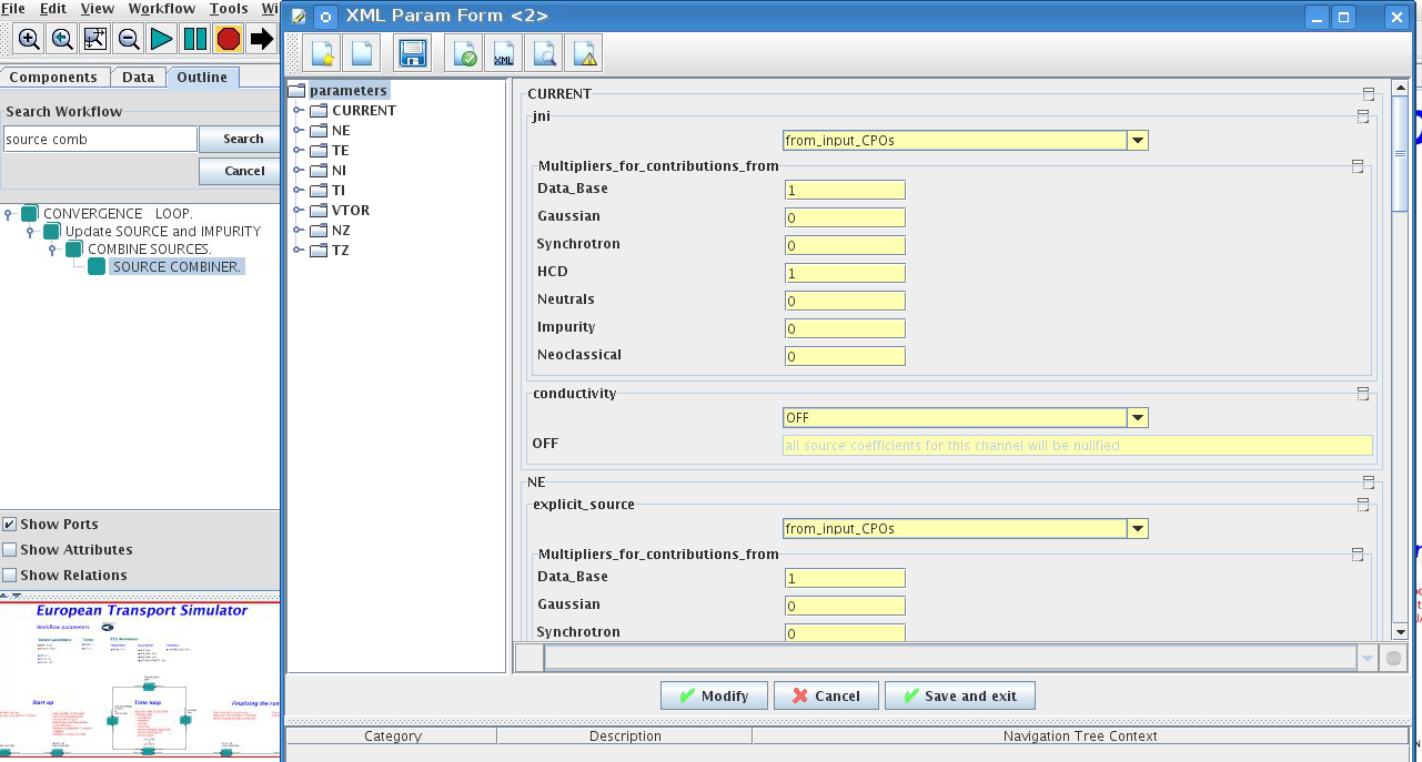
The fine tuning of of sources can be done through editing the XML code parameters of the source combiner actor:

• In the Outline browse for source combiner

• select Configure actor

• click Edit Code Parameters

• If you like the sources to the particular equation being activated - select from_input_CPOs, and then, put the multipliers against each contribution; if you select OFF contributions from all sources to this channel will be nullified.

• save and exit

• Commit

3.2.1.9. Instantaneous events & Actuators

At the moment, user can swith ON and OFF two types of events: PELLET and SAWTOOTH

3.2.1.9.1. Pellet

At the top level of the workflow you can configure times for pellet injection

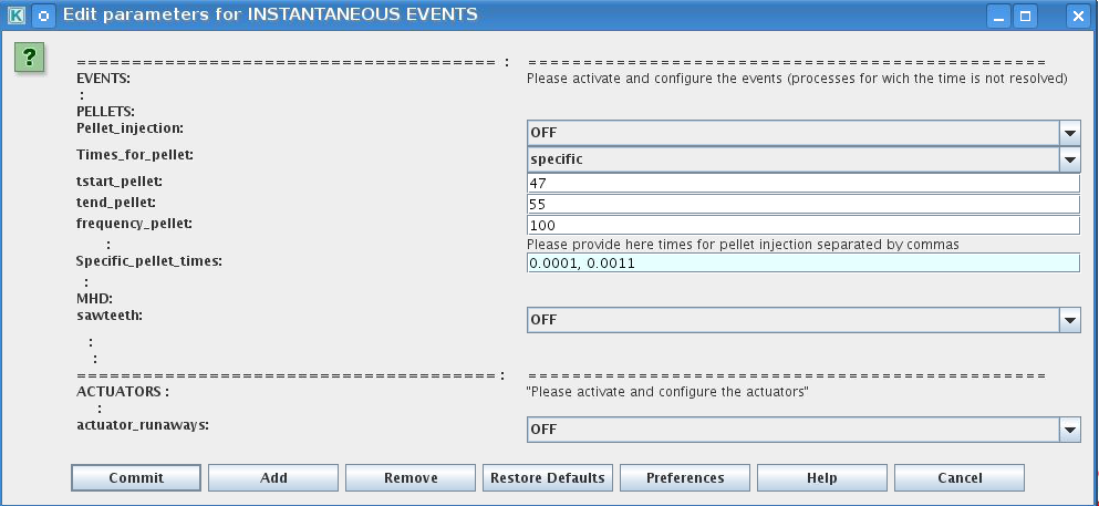
• right click on the box INSTANTANEOUS EVENTS & ACTUATORS

• select Configure actor to edit settings

• Select Pellet_injection equal ON if you like to use pellet in your simulation

• Select mode of operation:

  • Times_for_pellets equals specific – pellets will be shut at exact times specified in array times_pellet

  • Times_for_pellets equals frequency – pellets will be shut from tstart_pellet until tend_pellet with a frequency_pellet

• Commit

Parameters of individual pellet need to be configured through the code_parameters of the PELLET actor. To access it go to Outline on the right upper corner and open the following:

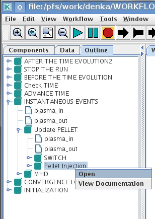
• right click on the actor PELLET

• select Configure actor

• click Edit Code Parameters

• edit parameters and click save and exit

• Commit

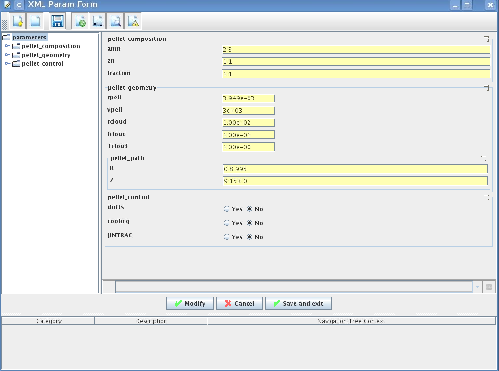
amn – atomic mass number: array of elements separated by space (1:nelements) [-]

zn – nuclear charge: array of elements separated by space (1:nelements) [-]

fraction – fraction of each element in the pellet, based on the number of atoms: array of elements separated by space (1:nelements) [-]

rpell – radius of the pellet [m]

vpell – velocity of the pellet [m/s]

rcloud – radius of the pellet cloud [m], radial extension of the cloud = 2*rp0

lcloud – length of the pellet cloud along the field line [m]

Tcloud – temperature of the pellet cloud [eV]

Pellet path is specified by two points, for which R and Z coordinated should be specified

R – R coordinates of the pivot and second points of the pellet path, separated by space [m]

Z – Z coordinates of the pivot and second points of the pellet path, separated by space [m]

Control switches allow to activate:

• drifts - YES - will activate radial displacement of deposition profile, same for all path points

• cooling - YES - will activate cooling of the other side of the plasma due to parallel heat transport (essential for large pellets, which might cross the same flux surface twice)

• JINTRAC - YES - will provide temperature reduction consistent with the model used in JETTO

3.2.1.9.2. Sawtooth

At the top level of the workflow you can switch ON/OFF possible MHD events

• right click on the box INSTANTANEOUS EVENTS & ACTUATORS

• select Configure actor to edit settings

• Select SAWTOOTH ON if you like to use them in your simulation

• Commit

3.2.1.9.3. Actuators

At the top level of the workflow you can switch ON/OFF actuator for Runaway Indicator (Runin) - this is ON by default. It only gives warning messages, and has no effect on the simulation results.

• right click on the box INSTANTANEOUS EVENTS & ACTUATORS

• select Configure actor to edit settings

• Select actuator_runaways OFF if you’d like not to use Runaway Indicator in your simulation

• Commit

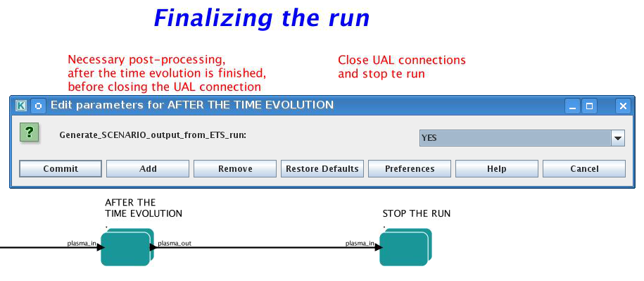
3.2.1.10. Scenario output

You can summarize the ETS run by activating the output to SCENARIO CPO (as post-processing of the run).

To activate the SCENARIO output:

• right click on the box AFTER THE TIME EVOLUTION

• select Configure actor

• select Generate_SCENARIO_output_from_ETS_run equal YES

• Commit

3.2.1.11. Visualization during the run

There is a number tools visualizing the ETS run.

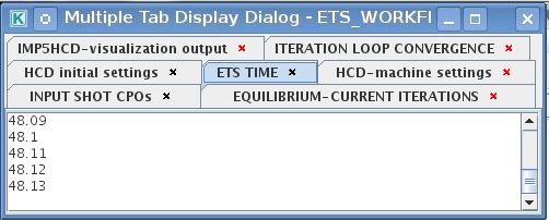
3.2.1.11.1. Multiple Tab Display

The display appeares automaticaly when the ETS workflow is launched. It displays diagnostic text messages from the workflow on following topics:

• Input data statement

• Iterations to check the initial convergence between EQUILIBRIUM and CURRENT

• Time evolution

• Convergence of iteratinos within the time step

• HCD settings

• Power used by HCD actors durung the run

Also the error messages from execution of the workflow will be displayed here.

3.2.1.11.2. ETSviz

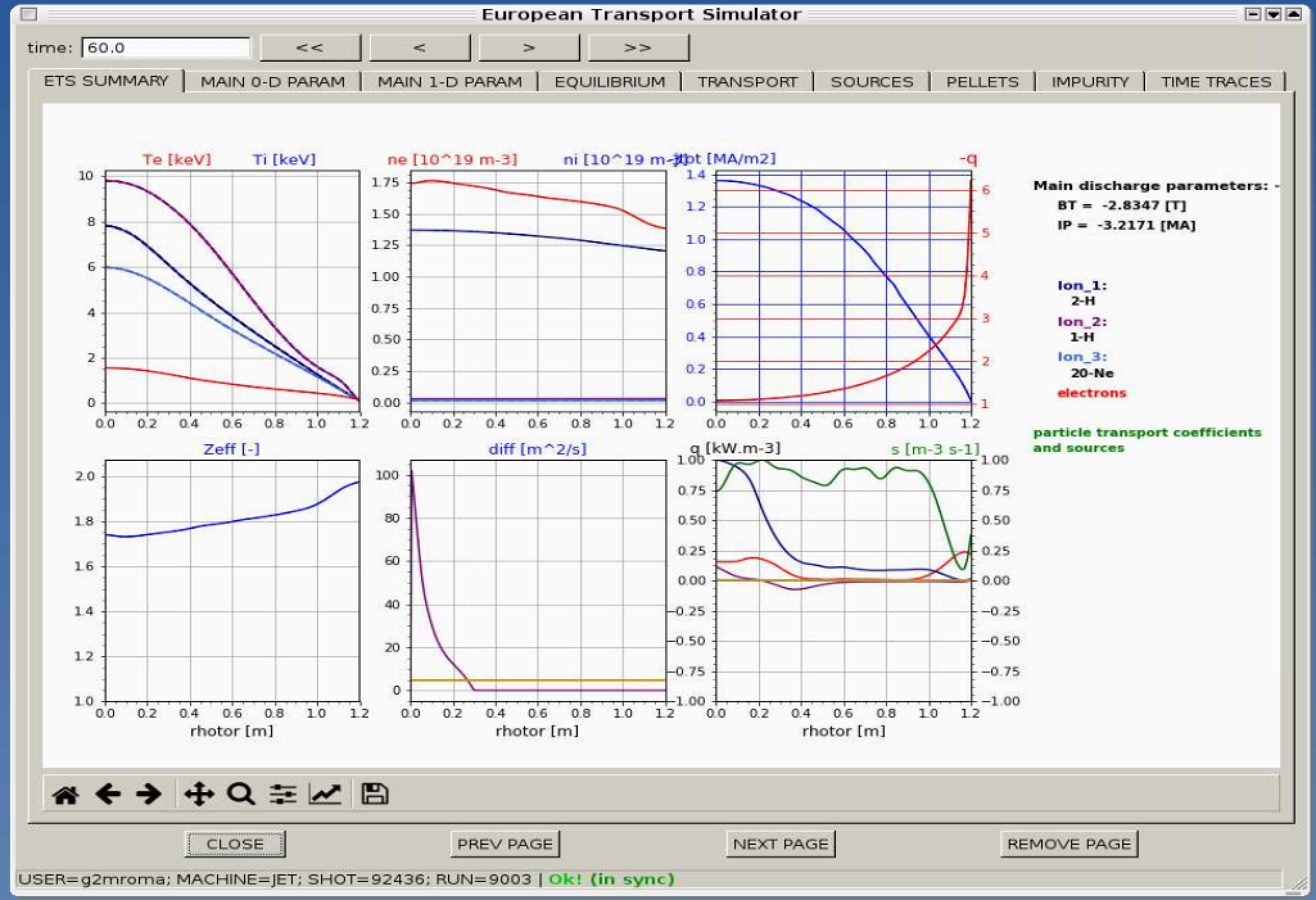
ETSviz is a python visualization tool with a graphical interphase that shows during the run the calculated kinetic profiles evolution, particle energy sources and sinks, equilibrium evolution and other useful infoirmnation. ETSviz appears automatically during the ETS run. If you would like to launch ETSviz you can find the script in $KEPLER/kplots

3.2.2. List of Actors

3.2.2.1. Equilibrium actors

Code name	Code Category	Contact persons	Short description
chease	Grad-Shafranov solver	Olivier Sauter	Chease is a fixed boundary Grad-Shafranov solver based on cubic hermitian finite elements see H. Lütjens, A. Bondeson, O. Sauter, Computer Physics Communications 97 (1996) 219-260
emeq	G-S solver	Rui Coelho	fix-b equilibrium
spider	G-S solver	Fable	ASTRA fix-B equilibrium
helena	G-S solver	Huijsmans	fix-B equilibrium
spider_imp12	G-S dolver	Coelho	ASTRA fix-b equilibrium

3.2.2.2. Core transport actors

Code name	Code Category	Contact persons	Short description
BohmGB	Bohm/gyro-Bohm transport coefficients	Taroni	Analytical model
CDBM	CDBM transport coefficients	Honda	Analytical model
Weiland	Transport coefficient from fluid turbulence	Pär Strand	Fluid model
GLF23	Transport coefficient from drift wave turbulence	Stabler (GA)	Gyrokinetic model
RITM	Transport coefficient from drift wave turbulence	Pär Strand	Gyrokinetic model
MMM	Transport coefficient from drift wave turbulence	PPPL	Gyrokinetic model
EDWM/EDWMZ	Transport coefficient from drift wave turbulence	Pär Strand	multi-ion model
nclass	Neoclassical transport coefficients	Pär Strand	Neoclassical model
neos	Neoclassical transport coefficients	Olivier Sauter	Neoclassical model
neowesz	Neoclassical transport coefficients	Bruce Scott	Neoclassical transport coefficients based on the expression in John Wesson’s book Tokamaks.
neoartz	Neoclassical transport coefficients	Bruce Scott
spitzer	Resistivity	Spitzer	Resistivity model
TGLF	Transport coefficient from drift wave turbulence	Stabler	Gyrokinetic model
NEO	Transport coefficient from drift kinetic equations	Belli	Gyrokinetic model
QualiKiz	Transport coefficient from drift wave turbulence	Citrin	Gyrokinetic model

3.2.2.3. Heating and current drive actors

Code name	Code Category	Contact persons	Short description
gray	EC/waves	Lorenzo Figini	GRAY is a quasi-optical ray-tracing code for electron cyclotron heating & current drive calculations in tokamaks. Code-parameter documentation can be found
travis	EC/waves	Nikolai Marushchenko and Lorenzo Figini	Travis is a ray-tracing code for electron cyclotron heating & current drive calculations in tokamaks.
Torray-FOM	EC/waves	Egbert Westerhof	Torray-FOM is a ray-tracing code for electron cyclotron heating & current drive calculations in tokamaks.
bbnbi	NBI/source	Seppo Sipila	Calculate the deposition rates of neutrals beam particles, i.e. the input source for Fokker-Planck solvers (not the heating and current drive). Note that the number of markers generated by BBNBI is described by the kepler variable number_nbi_markers_in.
nemo	NBI/source	Mireille Schneider	Calculate the deposition rates of neutrals beam particles, i.e. the input source for Fokker-Planck solvers (not the heating and current drive). Code-parameter documentation can be found
nuclearsim	nuclear/source	Thomas Johnson	Simple code for nuclear sources from thermal/thermal reactions. Code-parameter documentation can be found
afsi	nuclear/source	Thomas Johnson	Complete code for nuclear sources from all reactions. Code-parameter documentation can be found
nbisim	NBI, alphas/ Fokker-Planck	Thomas Johnson	Simple Fokker-Planck code calculating the collisional ion and electron heating from a particle source, either NBI or nuclear. Code-parameter documentation can be found
risk	NBI Fokker- Planck	Mireille Schneider	Bounce averaged steady-state Fokker-Planck solver calculating the collisional ion and electron heating from a particle source and the NBI current drive. Code-parameter documentation can be found
spot	NBI, alphas and ICRF Fokker -Planck	Mireille Schneider	Monte Carlo solver for the Fokker-Planck equation. Traces guiding centre orbits in a steady state magnetic equilibrium under the influence of Coloumb collisions and interactions with ICRF waves (through the RFOF library). The code can also be used for NBI and alpha particle modelling as it can handle source terms from the distsource CPO.
ascot4serial	NBI, alphas, ICRF/ Fokker-Planck	Otto Asunta/ Seppo Sipila	Monte Carlo Fokker-Planck solver calculating the collisional ion and electron heating from a particle source and the NBI current drive.
ascot4parallel	NBI, alphas, ICRF/ Fokker-Planck	Otto Asunta/ Seppo Sipila	Monte Carlo Fokker-Planck solver calculating the collisional ion and electron heating from a particle source and the NBI current drive.
Lion	IC / waves	Olivier Sauter and Laurent Villard	Global ICRF wave solver. Code-parameter documentation can be found
Cyrano	IC / waves	Ernesto Lerche and Dirk Van Eester	Global ICRF wave solver. Code-parameter documentation can be found
Eve	IC / waves	Remi Dumont	Global ICRF wave solver
StixReDist	IC / waves	Dirk Van Eester and Ernesto Lerche	1d Fokker-Planck solver for ICRF heating.
ICdep	IC / waves	Thomas Johnson	Generates Waves-cpo with an IC wave field with Gaussian deposition profiles described by a combination of antenna-cpo input and through code parameters input. Code-parameter documentation can be found
ICcoup	IC / coupling	Thomas Johnson	Simple model for the coupling waves from ion cyclotron antennas to the plasma. Code-parameter documentation can be found

3.2.2.4. Events actors

Code name	Code Category	Contact persons	Short description
pelletactor	pellet	Denis Kalupin
pellettrigger	pellet	Denis Kalupin
sawcrash_slice	sawteeth	Olivier Sauter
sawcrit	sawteeth	Olivier Sauter
runaway_indicator	runaway	Roland Lohneroch Gergo Pokol	Indicating the presence of runaway electrons: 1) Indicate, whether electric field is below the critical level, thus runaway generation is impossible. 2) Indicate, whether runaway electron growth rate exceeds a preset limit. This calculation takes only the Dreicer runaway generation method in account and assumes a velocity distribution close to Maxwellian, therefore this result should be considered with caution. The growth rate limit can be set via an input of the actor. Limit value is set to \( 10^{12} \) particle per second by default. (This growth rate generates a runaway current of approximately 1kA considering a 10 seconds long discharge.)

3.2.2.5. Non-physics actors

The ETS uses the following list of non-physics actors: addECant, addICant, backgroundtransport, calculateRHO, changeocc, changepsi, changeradii, checkconvergence, controlAMIX, coredelta2coreprof, correctcurrent, deltacombiner, emptydistribution, emptydistsource, emptywaves, eqinput, etsstart, fillcoreimpur, fillcoreneutrals, fillcoreprof, fillcoresource, fillcoretransp, fillequilibrium, fillneoclassic, filltoroidfield, gausiansources, geomfromcpo, hcd2coresource, ignoredelta, ignoreimpurity, ignoreneoclassic, ignoreneutrals, ignorepellet, ignoresources, ignoretransport, IMP4dv, IMP4imp, importimptransport, itmimpurity, itmneutrals, merger4distribution, merger4distsource, merger4waves, nbifiller, neoclassic2coresource, neoclassic2coretransp, parabolicprof, plasmacomposition, PowerFromArray, PowerModulation, profilesdatabase, readjustprof, sawupdate_slice, scaleprof, sourcecombiner, sourcedatabase, transportcombiner, transportdatabase, wallFiller and waves2sources.

3.3. Turbulent Flux Quantities in Transport Models

3.3.1. Overview

In conventional transport modelling, all quantities appearing in the equations are 1-D, in some radial coordinate (poloidal flux, normalised radius, etc). In general any monotonic radial coordinate is acceptable. In the TF-EU-IM, the toroidal flux radius is standard. All we need from the radial coordinate is the transformation to get to \(V,\) the volume enclosed by the flux surface, which is fundamental to the governing equations, which are conservation laws.

What we have to do is to take a measured result, which is a time-averaged fluctuation-based transport flux and turn it into 1-D quantities suitable to modelling. This is done using the flux surface average, explained in conventions. The transport equations themselves constitute a mean field approximation to the 3-D conservation laws. For the fundamentals encountered in transport modelling see R Hazeltine and J Meiss, Plasma Confinement (Addison-Wesley, 1992) chapter 8. For the special properties of transport driven by small-scale pressure driven ExB microturbulence see B Scott, “The character of transport caused by ExB drift turbulence,” Phys Plasmas 10 (2003) 963-976.

For ambipolarity we follow the rules for dynamical alignment, which follows the physics of how electron fluctuations determine the ExB velocity fluctuations, which then advect all species. Magnetic flutter nonlinearities act independently of this, but in our modelling they are used solely for heat fluxes since the averaged particle transport due to magnetic flutter and the current cancels, leaving the parallel ion velocity which we neglect for this purpose. The reference for dynamical alignment is B Scott, “Dynamical alignment in three species tokamak edge turbulence,” Phys Plasmas 12 (2005) 082305.

Note: there are now auxiliary actors provided for this purpose: IMP4DV, which does the D/V conversion and enforces ambipolarity assuming absence of impurities, and IMP4imp, which subsequently enforces ambipolarity for the set of main ion and impurity species. The IMP4DV actor should be invoked directly after the transport model actor in the workflow chain, if the model produces only fluxes or if the coefficients have to be modified with the flux given. Ambipolarity is done using IMP4imp if the coreimpurity CPO is used in the workflow.

3.3.2. Particle Flux as an Example

The mean field equation governing particle balance is the transport equation for electrons,

\[{\partial \over \partial t} \langle n \rangle + \langle \vec \nabla \cdot \widetilde n \vec {\widetilde v}_E \rangle = S\]

in which the tilde symbol over the n and v denotes fluctuating quantities and we neglect all transport processes except ExB eddy diffusion. The ExB velocity is given by

\[\vec v_E = {c \over B^2} \vec B \times \vec \nabla \phi\]

where \(\phi\) is the electrostatic potential.

The angle brackets denote the flux surface average, and we will use the property that the flux surface average of a divergence of a vector is the volume derivative of the flux surface average of a contravariant volume component of the vector, in this case

\[\langle \vec \nabla \cdot \vec \Gamma \rangle = {\partial \over \partial V} \langle \Gamma^V \rangle\]

where \(\Gamma\) is the particle flux whose flux-surface averaged volume component is

\[\langle \Gamma^V \rangle = \langle \widetilde n \widetilde v_E^V \rangle\]

This is converted to expression in terms of the radial coordinate ( rho` using the fact that both \(V\) and \(\rho\) are flux quantities whose gradients are parallel to each other. We have

\[{\partial \over \partial V} = {1 \over V'_\rho}{\partial \over \partial \rho}\qquad \Gamma^\rho = {1\over V'_\rho}\Gamma^V \qquad V'_\rho = {\partial V \over\partial \rho} \qquad g^{VV} = (V'_\rho)^2 g^{\rho\rho}\]

so we can write the transport equation as

\[{\partial n \over \partial t}+{1 \over V'_\rho}{\partial \over \partial \rho}V'_\rho \langle \Gamma^\rho \rangle = S,\]

where we have replaced \(\langle n \rangle\) with \(n\) following the assumptions of the 1-D version of mean field transport theory.

With all quantities now expressed in terms of flux quantities, we are free to characterise the transport flux \(\langle \Gamma^\rho \rangle\) in an arbitrary way, so long as only flux quantities appear. The flux expansion within the flux surface as well as expansion or contraction of surfaces of constant \(\rho\) is treated using the metric coefficient \(g^{ \rho \rho}\) which is dimensionless. This way we can characterise transport in terms of an effective diffusivity and an effective frictional slip velocity which are given in SI units. By convention both of these are done solely via \(g^{ \rho \rho}\) for convenience, also reflecting that the effective velocity is actually marking off-diagonal diffusive elements. Our convention for this follows the ETS code and is given by

\[\langle \Gamma^\rho \rangle = \langle g^{\rho \rho} \rangle \left( n V_{{\rm eff}} - D_{{\rm eff}}{\partial n\over \partial \rho} \right)\]

So despite the special spatial distribution of any particular transport process (ie, the underlying instability or nonlinear free energy access), the flux-surface averaged flux itself and its expression in terms of diffusion and frictional slip are identical characterisations.

3.3.3. Metric Coefficients

Transport modellers want the Ds and Vs as physical quantities in SI units. In general the fluxes are (magnetic) flux surface averaged quantities, which implies the existence of metric elements in the conversion. In our case we need \(\langle g^{\rho \rho} \rangle\) where \(\rho\) is the toroidal flux radius in meters, so the metric elements are dimensionless. In the equilibrium CPO, this is gm3 under equilibrium%profiles_1d in the structure.

Note this is different from the ASTRA code which casts the Vs as proper velocities, i.e., with one factor of grad-rho given by \(\langle \sqrt{g^{\rho \rho}} \rangle\) which is gm7 under equilibrium%profiles_1d in the structure. The units are the same and the informational content is the same, but this difference has to be taken into account in any transport modelling and benchmarking.

3.3.4. Heat Fluxes

The heat flux is treated in a similar way, with transport equation

\[{3 \over 2}{\partial p_e \over \partial t} +{1 \over V'_\rho}{\partial \over \partial \rho} V'_\rho \langle q_e^\rho \rangle = Q_e + \sum_{{\rm ions}}T_{ei},\]

for electrons, with \(T_{ei}\) giving the species transfer and \(Q_e\) the source. For ExB transport the heat flux has a advective (also called convective) and a conductive piece given by

\[q_E = q_E{}_{{\rm cond}} + (3/2) T \Gamma_E\]

which appears with a 3/2 due to the Poynting cancellation. For magnetic flutter transport the advective piece appears with the usual factor,

\[q_m = q_m{}_{{\rm cond}} + (5/2) T \Gamma_m\]

Here the forms are given for each species and \(E\) and \(m\) refer to the ExB eddy and magnetic flutter channels, respectively. For reasons given below we are neglecting the magnetic flutter piece \(\Gamma_m\) for the time being, and then the flutter piece merely adds to the heat diffusivity.

The forms of these due to the fluctuations are then

\[\langle q^\rho \rangle = (3/2) \langle \widetilde p \widetilde v_E^\rho \rangle + \langle \widetilde q_\parallel \widetilde b^\rho \rangle\]

which breaks into advective and conductive pieces according to linearisation of the pressure fluctuations

\[\langle q_{{\rm cond}}^\rho\rangle = (3/2) n \langle \widetilde T \widetilde v_E^\rho\rangle + \langle \widetilde q_\parallel \widetilde b^\rho\rangle \qquad\qquad \langle q_{{\rm adv}}^\rho \rangle = (3/2)T \Gamma = (3/2)T\langle\widetilde n \widetilde v_E^\rho \rangle\]

hence the density fluctuation piece is accounted for by the particle flux. Neglect of the magnetic flutter advective piece (and particle flux) is the same as neglect of the \({\widetilde u_\parallel} {\widetilde b^ \rho}\) nonlinearity (in the delivery of the results, not in the turbulence computations themselves).

The total conductive flux is then represented by

\[\langle q_{{\rm cond}}^\rho \rangle = \langle g^{\rho \rho} \rangle \left( nTY_{{\rm eff}} - n \chi_{{\rm eff}}{\partial T \over \partial \rho} \right)\]

with \(\chi\) and \(Y\) giving the heat diffusion and frictional slip pieces for each species, respectively (these are in diff_eff and vconv_eff in the CPO for each quantity).

Operationally, the turbulence module communicates the diff_eff and vconv_eff due to each transport channel for each species to the transport solver, and the metric coefficients are used by both modules. The two modules can be on arbitrarily different grids, which communicate through standard interpolation. This despite the fact that transport at the micro-level is angle dependent (in general, it can be 3-D in the time average if the sources are 3-D). The effective transport is 1-D so long as parallel sound transit within the flux surface remains fast compared to the local transport time. This breaks down anyway in the edge, so the fact that the volume is a problematic coordinate and the flux surface average is a problematic operation on open field lines doesn’t enter.

3.3.5. Ds and Vs from Turbulence Codes to Transport Solvers

To serve the results from turbulence codes to transport solvers, we have to turn the fluxes (results) into diffusivities and effective velocities (coefficients, Ds and Vs for short), which represent more information than is at hand. Transport solvers must work with Ds and Vs because they use implicit schemes. The matrix must be diagonally dominant; hence one cannot simply use the Vs. Fluxes which are zero and/or negative should be given with positive diffusivities for the solvers to work. We need a set of rules to provide this.

Considering the particle and heat transport fluxes for a given species, we convert the gradient in to a logarithmic derivative and express the flux in terms of a specific flux, which has units of velocity,

\[\begin{split}F &= \frac{1}{n} \langle g^{\rho\rho}\rangle^{-1} \langle \Gamma^\rho \rangle= V_{{\rm eff}} - D_{{\rm eff}}\frac{\partial \log n}{\partial \rho}\\ G &= \frac{1}{nT} \langle g^{\rho \rho} \rangle^{-1} \langle q^\rho_{{\rm cond}}\rangle = Y_{{\rm eff}} - \chi_{{\rm eff}}\frac{\partial \log T}{\partial \rho}\end{split}\]

wherein the conductive part of the heat flux (without the \(3 \Gamma / 2\) enters.

The choice of what to do with the Ds and Vs is somewhat arbitrary. The needs of implicit transport solvers is for a positive D regardless of the value or sign of either flux. We decide this by putting a limit on the effective Prandtl number or its inverse: the larger specific flux is taken to be entirely diffusive, with the effective velocity set to zero. Furthermore, to address cases with very small or negative gradients, we use proxy variables for the scale lengths to calculate the provisional diffusivities before using the Prandtl number limitation to turn these into actual diffusivities. Finally, the rest of the flux is asigned to the effective velocity, so that the D and V formula reflects the actual specific flux.

The Prandtl number limitation is expressed as follows. If the smaller specific flux is within a factor of 5 of the larger, then both are purely diffusive and the effective velocities are both zero. If not, then the D ratio is set to 5, with the result that the smaller D, having been corrected, is accompanied by the corresponding V, which is now nonzero. The specific flux with the larger D will be returned with a V which is zero.

The rationale is that the turbulent mixing by the ExB velocity affects all processes, but that linear forcing can shift the average phase shift of the fluctuations such that the effective flux can be small or negative. The simplest example is adiabatic electrons, for which the ion heat flux is robust but the particle flux is zero. In most situations the specific heat flux will be the larger, and hence the familiar situation is that of a D and V for the particle flux but a D (the chi) only for the conductive heat flux.

The full algorithm starting with the specific fluxes appears as

\[\begin{split}L_n^{-1} &= \max \left( {1 \over R}, \left\vert {\partial \log n \over \partial \rho} \right\vert \right) \quad L_T^{-1} = \max \left( {1 \over R},\left\vert {\partial \log T \over \partial \rho} \right\vert \right)\\ D' &=\left \vert F \right \vert L_n \quad \chi' = \left \vert G \right \vert L_T \\ D &= \max \left( D', {1\over 5} \chi' \right) \quad \chi = \max\left( \chi', {1 \over 5} D' \right) \\ V &= \left( F + D {\partial \log n \over \partial \rho} \right) \quad Y = \left( G + \chi \frac{\partial \log T}{\partial \rho} \right)\end{split}\]

and all four elements are set. Note that the channels are done in parallel except for the Prandtl correction, in which the Max’s are taken sequentially. For the provisional diffusivities, absolute values are used to ensure positive values which are needed by transport solvers.

Note how in the end the actual gradients are used. If the gradients are moderate then their actual values are used, and if the Prandtl correction is not invoked, then both channels are diagonal. In any case the full relation is used to get the effective velocities (V and Y) so having set the rules to handle the arbitrariness of the diffusivities (D and chi) to guarantee reasonable diagonal dominance in a transport solver, the D’s and V’s agree with the fluxes themselves.

If there are more than two specific fluxes per species to consider, then we treat each scale length separately as above and use N-way maxima in the Prandtl correction for the N channels.

3.3.6. Ambipolarity

There remains the issue of ambipolarity of the D and V for particle flux. For a pure singly charged plasma the ion and electron Ds and Vs should be equal. Even if the turbulence model is gyrokinetic or gyrofluid, in which case the gyrocenter charge density is not zero but is equal to the generalised vorticity (polarisation), the quantities given to a transport solver should follow the rules for a fluid representation. However, transport modelling usually applies ambipolarity rules to the electrons after computing the ions, while the action of turbulence is actually the other way around: Dynamical alignment refers to the process by which (1) electron parallel dynamics controls the electrostatic fluctuations, then (2) the resulting ExB velocity advects all species equally. So we correct the particle fluxes by assuming the electrons determine the D according to the above procedure and then (1) the fluctuations in the flux-inducing part of the spectrum for the logarithmic densities are the same, and (2) the D’s are the same. Then the V’s are solved for again, by taking

\[D_z = D_e = D \qquad \qquad V_z = V_e + D {\partial \log b_z \over \partial \rho} \qquad \qquad b_z = n_z/n_e\]

This is better than the transport modelling convention but will give them the same information in a different way, and they will compute ambipolar particle fluxes (radial transport of charge is zero).

3.3.7. Statistical Character

Turbulence has a statistical character, so convergence to a mean is not monotonic and when within one std dev of the mean there is no further convergence. The diffusivity for ExB turbulence is comparable to

\[D_E = \left. \langle (\widetilde v_E)^2 \rangle \right / \langle (\varpi)^2 \rangle^{1/2} \qquad \qquad \varpi_E = {c \over B} \nabla_\perp^2 \widetilde \phi\]

where \(\varpi_E\) is the ExB vorticity fluctuation, and these angle brackets denote the ensemble average. To get an ensemble average over a statistical quantity in practice, one must do some sort of finite-time running averaging.

For transport modelling, the transport coefficients derived from a turbulence code should always be given in terms of running exponential averages.

3.4. Running Exponential Average

3.4.1. Overview

In conventional transport modelling, turbulent fluxes are modelled in terms of processes which are diffusive in the local relaxation sense, with the average flux given by a diffusion coefficient and an effective pinch velocity. The equations are of dominantly parabolic character, which means in practice that an iterate will move monotonically towards the solution in parameter space.

This is not the case for turbulence. Convergence is statistical, which is something different than a diffusive relaxation. If turbulence is stationary, it is meant only that the mean of a distribution of iterates is stationary, not the iterates themselves. The standard deviation can be significant, of order unity compared to the mean, of any distribution of iterates.

This makes for a noisy signal if the output of a turbulence code is used for transport coefficients in a workflow. A sound way to overcome the attendant problems is to use a moving average. Even an average over a moving window can be as noisy as the original signal, however. What works better is a weighted average over recent past values. A method to get this is called a running exponential average, which is essentially the same thing as a convolution integral over an exponential memory decay times the past signal. It turns out to be very easy to obtain this without saving past values.

The original reference for the following is S W Roberts, “Control Chart Tests Based on Geometric Moving Averages,” Technometrics 1 (1959) 239-250, cited by all the good WWW resources, including the Wikipedia page on Moving Averages and the NIST Statistical Handbook online.

3.4.2. Definition

Consider a process \(p ( \vec u )\) which is a functional of dependent variables \(\vec u\). Measure \(p\) at discrete time intervals \(t_n,\) with values \(p_n=p(t_n)\) and interval length \(\tau=t_n-t_{n-1}\). The moving exponential average \(A_n=A(p_n)\) on the \(n \hbox{-th}\) interval is defined as

\[A_n = \epsilon p_n + (1-\epsilon)A_{n-1} \qquad \qquad \hbox{with} \qquad \epsilon=\alpha \tau\]

in which the small parameter \(\epsilon\) is given in terms of the interval \(\tau\) and an inverse time constant \(\alpha.\)

In the first instance \(p\) is measured there is no \(A\) so the first value of \(A\) is simply set to \(p\) since it can be assumed that the initial state for \(p\) has persisted for infinite previous time up to the initial time point.

3.4.3. Differential Equation

The equivalent differential equation is found by forming the relevant finite difference,

\[A_n - A_{n-1} = \epsilon (p_n - A_{n-1})\]

which we can also cast as

\[(1-\epsilon)(A_n - A_{n-1}) = \epsilon (p_n - A_n)\]

Taking the limit \(\tau \to 0\) is the same as taking \(\epsilon \to 0\) so both of these expressions become equivalent to

\[{\partial A \over \partial t} = \alpha(p-A)\]

whose solution is given below.

3.4.4. Equivalence to Past-Time Convolution Integral

The solution of the above differential equation is given by the method of undetermined coefficients,

\[{\partial A \over \partial t} +\alpha A = \alpha p \ \ e^{-\alpha t}{\partial \over \partial t} \left( e^{ \alpha t} A \right) = \alpha p \ \ {\partial \over \partial t} \left( e^{\alpha t} A \right) = \alpha p e^{\alpha t}\]

We may integrate this over all past time, to find

\[A(t) = \int_{-\infty}^t \alpha dt' p(t') e^{-\alpha (t-t') }\]

This is a convolution integral over the kernel \(e^{-\alpha(t-t')}\) and the signal \(p(t')\). The time constant \(\alpha^{-1}\) is just the memory decay time, while if \(p\) is constant then the integral yields unity times \(p\). This is the same as the normalisation with the \((1-\epsilon)\) factor in the average formula above, which is needed since the interval is of finite size.

Hence the running exponential average is operationally the same as a memory decay integral over past time. The elegant feature is the need to keep only the current value of \(A\), as it already contains all that is needed of the past time evolution of \(p\).

3.4.5. notes

Some properties of the running exponential average and how to choose its main time-memory parameter:

• The \((1-\epsilon)\) factor is needed for normalisation

• if \(p=\hbox{constant}\) then \(A=p\) for all \(t\)

• the integral with \(\alpha dt'\) yields unity

• the \(\epsilon\) and \((1-\epsilon)\) factors add to unity

• therefore set the first value of \(A\) to the first value of \(p\)

• in choosing the memory decay time \(\alpha^{-1} \dots\)

• one should have \(\alpha \tau_{cor} \ll 1\)

• best results are for \(\alpha \tau_{sat} \sim 1\)

• some trial/error required; edge turbulence likes \(\alpha^{-1}=200 L_\parallel / c_s\)

In these expressions \(\tau_{{cor}}\) and \(\tau_{{sat}}\) are the correlation and saturation times of the turbulence, respectively.